Simulation of the movement of an electric vehicle according to the WLTC cycle
This example will demonstrate the simulation of the movement of an electric vehicle according to the WLTC driving cycle. The parameters of the car, electrical and mechanical systems repeat the characteristics of an electric vehicle like the Nissan Leaf.
Description of the parameters and structure of the model
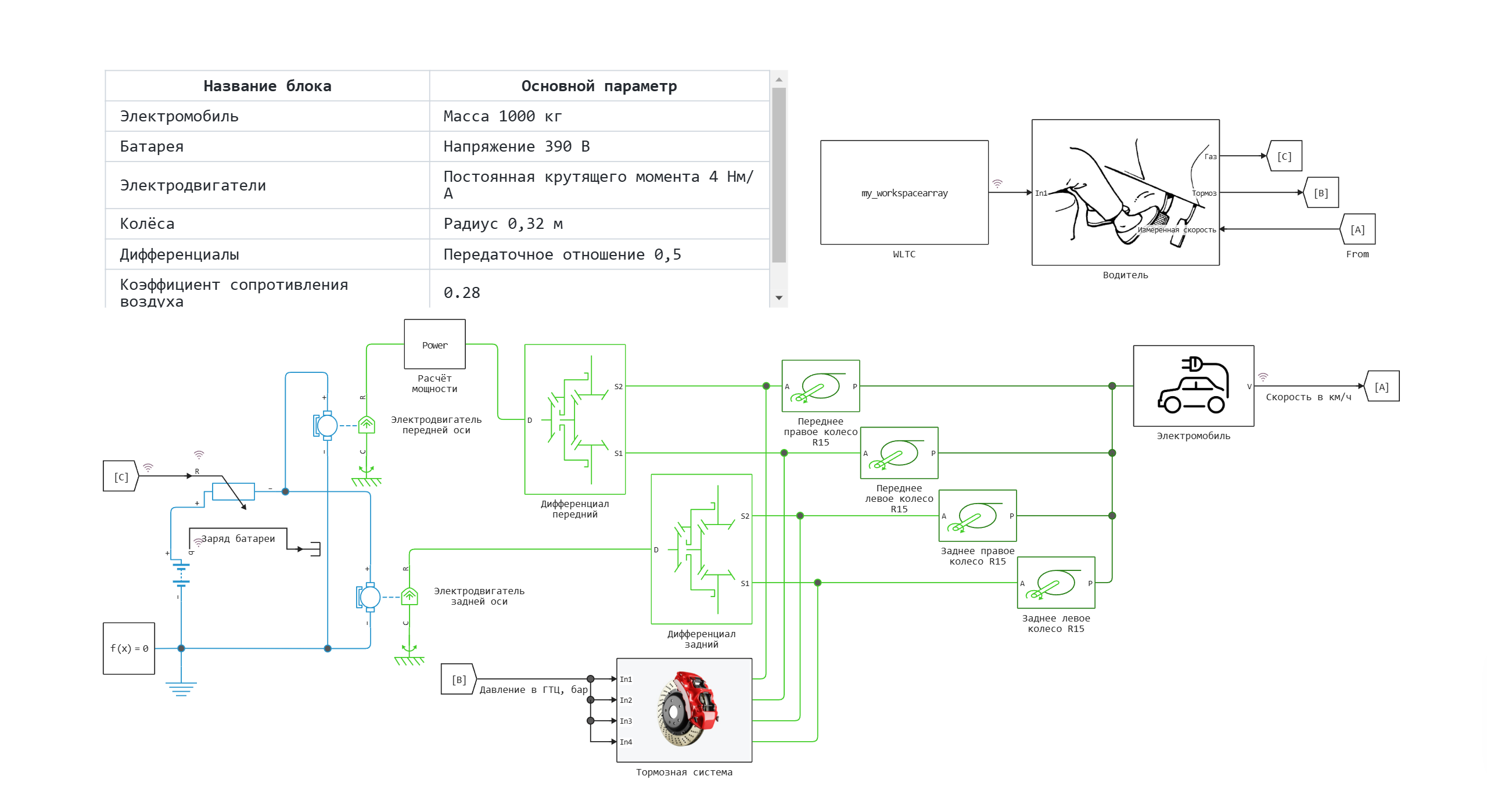
The movement of an electric vehicle and its inertia are described by the block Electric vehicle. The resulting force from two pairs of wheels connected to gearboxes and electric motors that convert and generate torque comes to the left port of this unit. The air resistance force is also calculated in the unit.
The main parameters of the model:
| Block name | The main parameter |
|---|---|
| Electric vehicle | Weight 1000 kg |
| Battery | Voltage 390 V |
| Electric motors | Torque constant 4 Nm/A |
| Wheels | Radius 0.32 m |
| Differentials | Gear ratio 0.5 |
| Air resistance coefficient | 0.28 |
Model diagram:
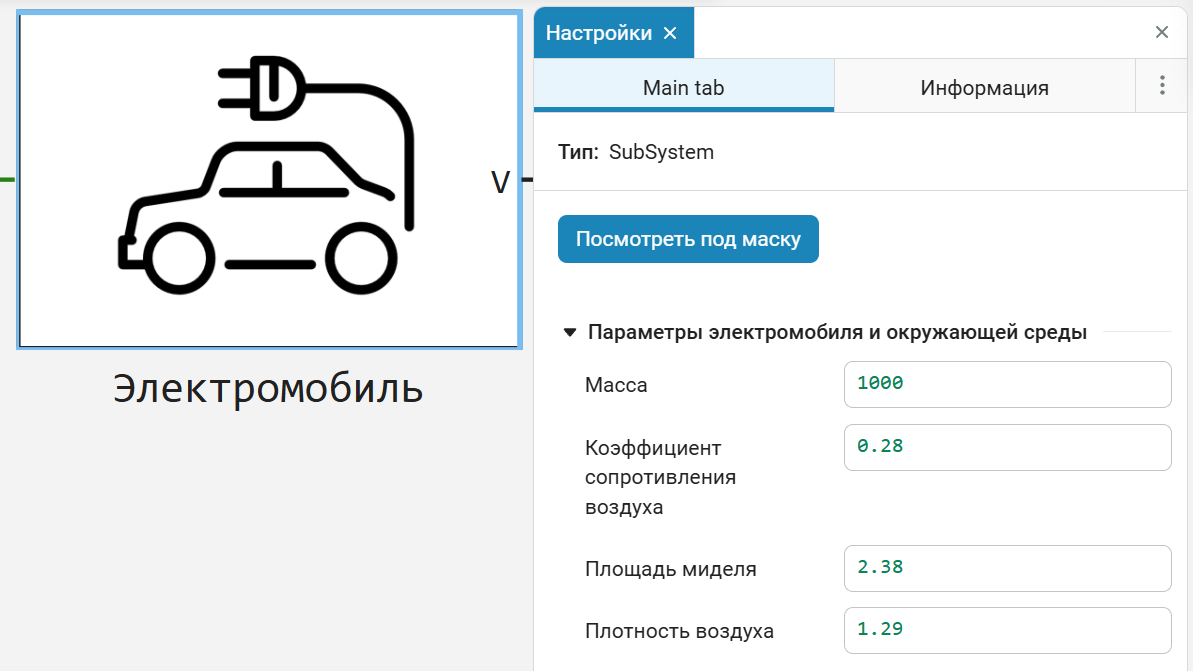
The Electric Vehicle unit
Subsystem diagram Electric vehicle:
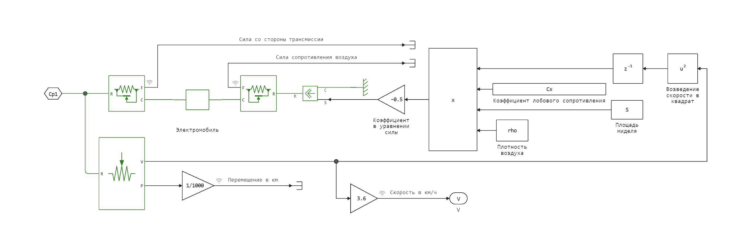
The air resistance force in this subsystem is determined by the formula:
where: - drag coefficient, - air density, , - the area of the midsection (the largest cross-sectional area of the object perpendicular to the direction of movement), , - the speed of the electric vehicle.
The main parameters defined in the subsystem Electric vehicle:
The Driver subsystem diagram:
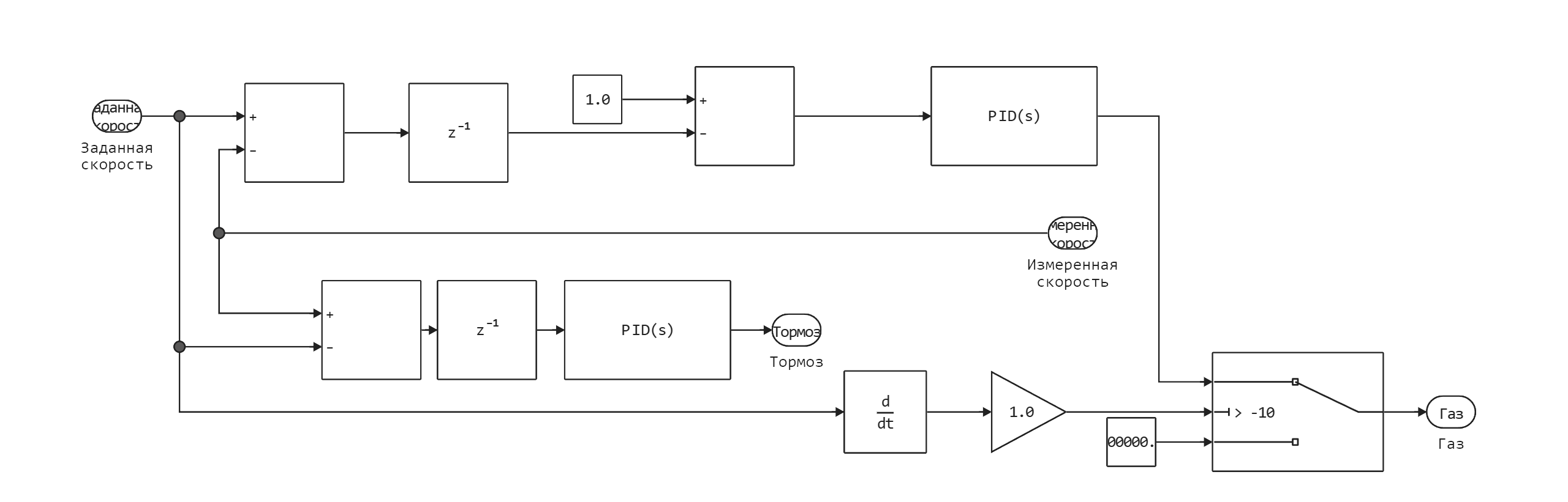
The Driver subsystem is a control system that generates control signals for actuators, which are brakes and electric motors of an electric vehicle. Electric motors are represented by blocks Front axle electric motor and Rear axle electric motor, and brakes by block Braking system. In the Add block, a mismatch signal is calculated between the set and measured speeds, which is then sent to the PID controllers that generate control signals.
Subsystem diagram of the braking system:
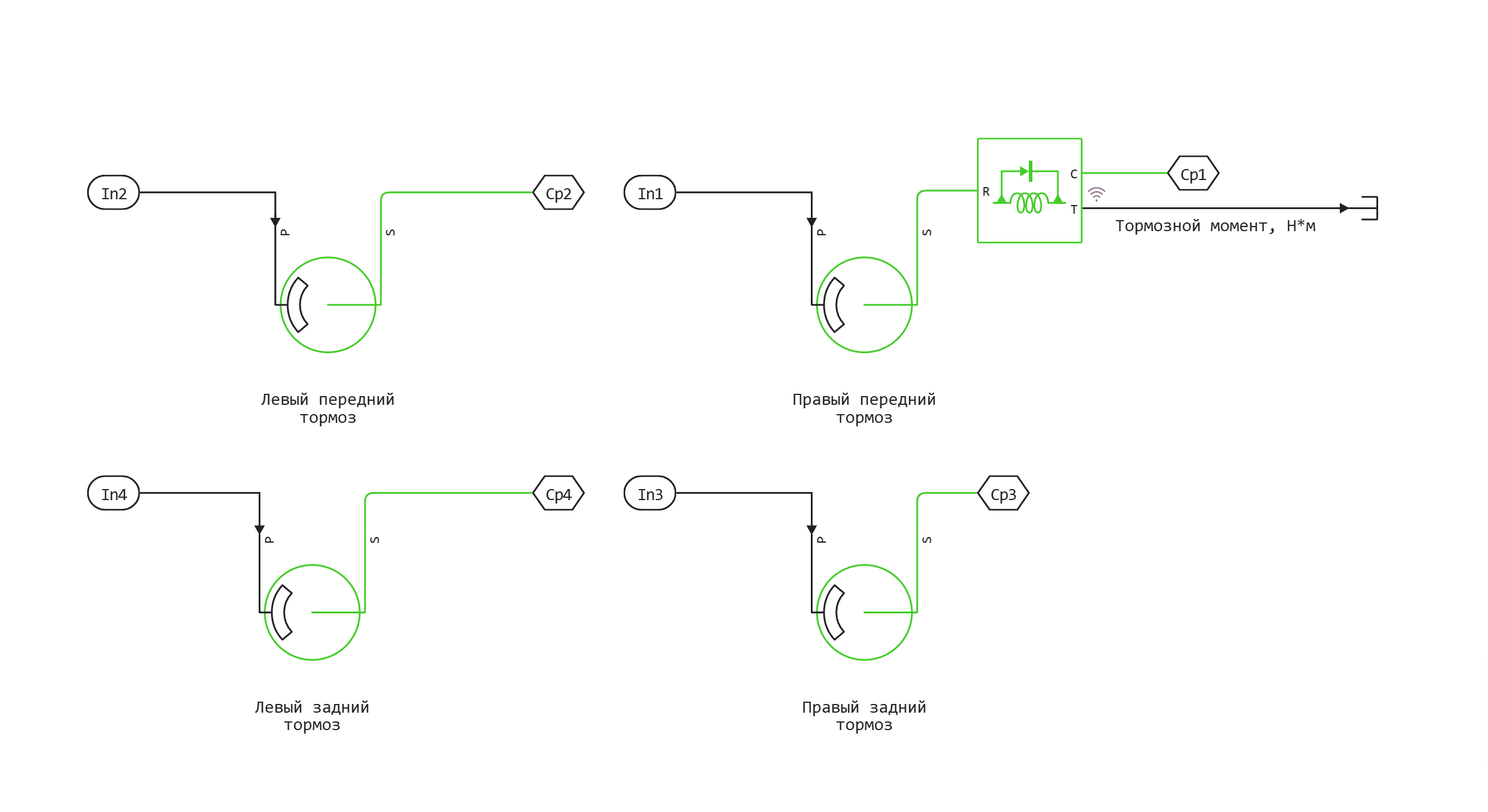
The subsystem consists of 4 brake discs. The input signal coming to port P determines the pressure in the braking system, port S transmits the braking torque to each of the wheels.
The WLTC block
The WLTC block is a From Workspace block that receives data about the WLTC driving cycle converted from XLSX format from the model's callbacks.
Defining the function to load and run the model:
function start_model_engee()
    try
        engee.close("electric_vehicle_performance", force=true) # closing the model
        catch err # if there is no model to close and engee.close() is not executed, it will be loaded after catch.
            m = engee.load("$(@__DIR__)/electric_vehicle_performance.engee") # loading the model
        end;

    try
        engee.run(m) # launching the model
        catch err # if the model is not loaded and engee.run() is not executed, the bottom two lines after catch will be executed.
            m = engee.load("$(@__DIR__)/electric_vehicle_performance.engee") # loading the model
            engee.run(m) # launching the model
        end
end
Running the simulation
start_model_engee() # running the simulation using the special function implemented above
Recording of signals received during the simulation from simout to variables (there is a lot of data, the process can take about 4 minutes):
t = simout["electric_vehicle_performance/Electric vehicle/Speed in km/h"].time[:]; # time
T = simout["electric_vehicle_performance/Power calculation/Electric motor torque"].value[:]; # electric motor torque
speed = simout["electric_vehicle_performance/Electric vehicle/Speed in km/h"].value[:]; # vehicle speed
forces_left = simout["electric_vehicle_performance/Electric vehicle/Power from the transmission side"].value[:]; # forces acting on the vehicle from the transmission side
forces_right = simout["electric_vehicle_performance/Electric vehicle/Air resistance force"].value[:]; # forces acting on the car from the environment
w = simout["electric_vehicle_performance/Calculation of power/Motor speed"].value[:]; # electric motor rotation speed
q = simout["electric_vehicle_performance/Battery charge"].value[:]; # battery charge
P = simout["electric_vehicle_performance/Power calculation/Electric motor power, kW"].value[:]; # electric motor power
WLTC1 = simout["electric_vehicle_performance/WLTC.1"].value[:]; # The WLTC cycle
pos = simout["electric_vehicle_performance/Electric vehicle/Movement in km"].value[:]; # moving an electric vehicle
;
Visualization of simulation results
Launching the charting library:
using Plots
gr()
Plotting the forces acting on an electric vehicle and its speed:
p1 = plot(t, forces_left, label="Force from the transmission, N", linewidth=2)
p2 = plot(t, forces_right, label="Air resistance, N", linewidth=2, linecolor=2)
p3 = plot(t, speed, label="Speed, km/h", linewidth=2, linecolor=3)
plot(p1, p2, p3, layout=(3,1))
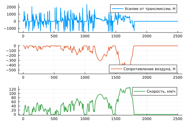
The analysis of force graphs allows us to conclude that the stages of the high-speed driving cycle make the greatest contribution to energy consumption. This is due to the fact that the aerodynamic drag force acting on an electric vehicle increases in proportion to the square of the speed.
Plotting the torque, speed, and power of an electric motor:
p1 = plot(t, T, label="Torque, NM", linewidth=2)
p2 = plot(t, (w * 9.55), label="Rotation speed, rpm", linewidth=2, linecolor=2)
p3 = plot(t, (T .* w ./1000), label="Power, kW", linewidth=2, linecolor=3)
plot(p1, p2, p3, layout=(3,1))
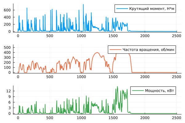
As the car accelerates, the torque decreases and the rotation speed of the electric motor increases. The mechanical power produced by this electric motor increases as the force of air resistance increases, depending on the speed.
The power of the electric motor is calculated using the formula:
where - the torque, in , and - rotation speed, in .
Graph of measured and set speed:
plot(t, speed, label="Measured speed, km/h", linewidth=2)
plot!(t, WLTC1, label="Set speed, km/h", linewidth=2)
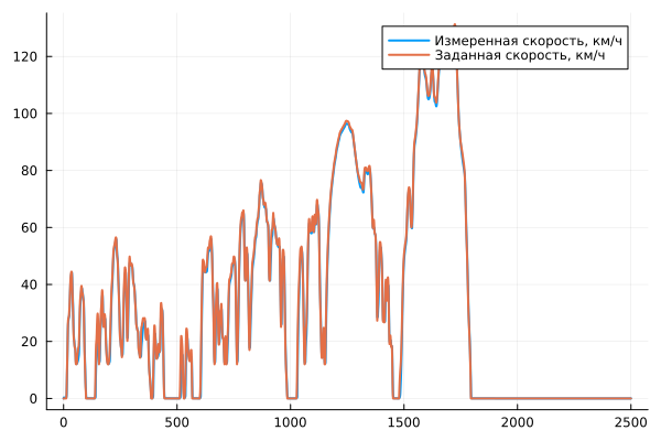
The graph shows that the electric car adheres to the set speed with small deviations. You can reduce these deviations by fine-tuning the controls in the unit. The driver.
Graphs of electric vehicle movement and battery charge:
p1 = plot(t, pos, label="Electric vehicle movement, km", linewidth=2)
p2 = plot(t, (q * 0.0002777777777778), label="Battery charge, Ah", linewidth=2)
plot(p1, p2, layout=(2,1))
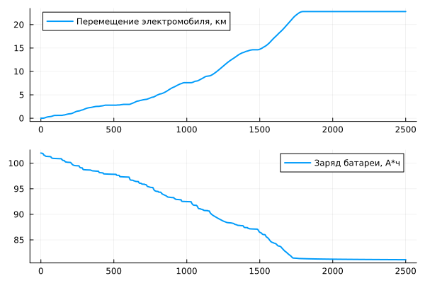
By analyzing the graphs of battery charge and movement of an electric vehicle, you can calculate how much energy was spent on overcoming the path.:
println("Energy spent on one driving cycle: ", round(maximum(q * 0.000277) - minimum(q * 0.000277), digits=3), " A*h")
By simple calculations, you can estimate the driving range of an electric car on one full battery charge.:
total_tange = maximum(q * 0.000277) / (maximum(q * 0.000277) - minimum(q * 0.000277)) * maximum(pos)
println("Electric vehicle power reserve: ", round(total_tange, digits=3), " km")
println("Specific energy consumption: ", maximum(q * 0.000277) / total_tange, " A*h/km")
Conclusion:
This example demonstrates the simulation of the movement of an electric vehicle according to the WLTC driving cycle. Calculations of productivity, in particular power reserve and specific energy consumption, have been carried out. The model can be refined by additional parameterization of the blocks and by adjusting the controls. Other driving cycles can also be loaded into the From Workspace block, which can be used to evaluate the performance of an electric vehicle in different conditions.