Assessment of the effect of the gain factor on the stability margin
This example shows how to study the effect of the gain factor on the stability margin and on the response characteristics of a closed-loop control system.
Stability of a closed system
Stability usually means that all internal signals remain limited. This is a standard requirement for control systems to avoid loss of control and damage to equipment. For linear feedback systems, stability can be estimated by looking at the poles of the closed loop transfer function. Let's consider a system with the following structural scheme:
Assume that the gain factor is . Let's define a description of the closed loop transfer function using the library ControlSystems.jl.
Pkg.add(["ControlSystems"])
using ControlSystems
G = tf([.5, 1.3],[1, 1.2, 1.6, 0]);
T = feedback(G,1)
We get the poles of the system.
pole(T)
A closed system at It is stable because all poles have negative real values.
How stable is the system?
Checking the poles of a closed loop gives us an idea of stability. In practice, it is more useful to know how stable or unstable the system is. One of the indicators of reliability is how much the gain of the circuit can change before stability is lost. To do this, you can use the root hodograph graph to estimate the range of values. , for which the system is stable:
plot(rlocus(G))
The asymptote marked in blue intersects the real axis (Y-axis) at the point with the value . You can hover over the chart and verify this. From this we can conclude that if the gain factor is in the range then the system will be stable.
Amplitude and phase margin
Changes in the gain factor in the circuit are just one aspect of stability. In general, imperfect modeling of the control object means that both the gain and the phase are not precisely known. Since modeling errors are most dangerous near the cutoff frequency (the frequency at which the open-loop gain is 0 dB), it is also important how acceptable a phase change is at this frequency.
The phase margin shows how much the phase can change before the stability is lost. Similarly, the amplitude margin indicates which gain change is necessary at the cutoff frequency in order to lose stability. Together, these two indicators provide an estimate of the "margin of stability" for closed loop stability. The smaller the stability limits, the more fragile stability is.
We will build a housing and communal services complex with reserves of stability. You can determine the reserves of stability using the function marginplot().
marginplot(G)
The amplitude margin in this case is about 9 dB. You can hover the cursor over the intersection point of the wind line and the roof, and make sure of this. The limits of the stability of the system can be seen above the graph. However, it must be borne in mind that the limit of stability in amplitude is They are expressed as a limit value of the gain, not in dB.
The phase margin (Pm) is about 45 degrees.
Consider the system's response to a step signal.
S1 = stepinfo(step(T,25));
plot(S1)
The overshoot in this case is 21% and there will be some fluctuations.
We will increase the gain factor by 2 times. We introduce the values of the stability reserves by the function margin() and we will construct a transitional characteristic.
M = margin(2*G)
GmdB = 20*log(10,M.gm[1][1])
Pm = M.pm[1][1]
display(GmdB)
display(Pm)
To derive the characteristics of the transient process, we use the function stepinfo(). Parameters such as steady-state time, overshoot, and so on will be reflected on the graph using plot().
S2 = stepinfo(step(feedback(2*G,1),60));
plot(S2, title = "Closed-loop reaction at k=2")
We see on the LFCH that the phase margin (Pm) has decreased, overshoot and steady-state time (setting time) have increased. This indicates that we are approaching an unstable situation.
Systems with multiple reserves of amplitude resilience
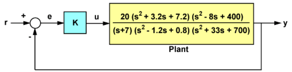
Some systems have several amplitude stability reserves or several phase transitions through 180 degrees. For example, consider the following block diagram.
.png)
The transient process of a closed system in this case comes to a steady value - the system is stable.
G1 = tf([20],[1, 7]) * tf([1, 3.2, 7.2],[1, -1.2, 0.8]) * tf([1, -8, 400],[1, 33, 700]);
T1 = feedback(G1,1);
plot(step(T1,7), title = "Closed-loop reaction at K=1")
To assess how stable this system is , we will build the LCH and LFCH systems.
marginplot(G1)
Note that there are two 180 degree phase transitions with corresponding gain values of -9.35 dB and +10.6 dB. Negative values of the gain factor indicate a loss of stability when the gain is reduced. While positive gain values indicate a loss of stability as the gain increases. This is confirmed by plotting the stepwise response of a closed loop to change the gain $\pm$6 dB at k=1:
k2 = 2;
T2 = feedback(G1*k2,1);
k3 = 1/2;
T3 = feedback(G1*k3,1);
step([T1 T2 T3],12)
plot(step([T1 T2 T3],12), label = ["K = 1" "K = 2" "K = 0.5"])
The graph shows an increase in fluctuations with both lower and higher gain values.
Conclusion
Thus, we have considered the effect of the gain factor on the stability of a closed loop and the margin of amplitude stability, in particular.