Identification of a control system object with a fuzzy PID controller
In this example, two tasks are solved at once. First, we identify the control object based on experimental data. Secondly, we are implementing a fuzzy output system for the PID controller.
EngeePkg.purge()
Pkg.add(["ControlSystemIdentification", "FuzzyLogic"])
using ControlSystemIdentification, FuzzyLogic
Let me remind you that the identification workflow looks like this:
-
Collecting experimental data
-
Choosing the model structure
-
Identification of the model
-
Validation of the model
Identification of the management object
Collecting experimental data from the management facility
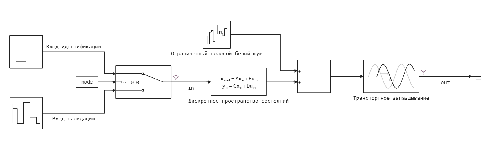
The simulation of the experimental installation of the control facility is presented in the plant.engee model. The control object is a discrete system with one input and one output. Noise and a slight delay have also been added to the model.
The identification of the object will be carried out by a transitional process, for this we will provide a step at the entrance of the system.
Let's record the identification data.:
mode = 1; # Recording identification data
if "Plant" in [m.name for m in engee.get_all_models()]
    m = engee.open( "Plant" ) # loading the model
else
    m = engee.load( "Plant.engee" )
end
results = engee.run(m, verbose=true)
dataout = collect(results["out"]);
datain = collect(results["in"]);
# Sampling rate of the system from the time vector
Ts = dataout.time[2] - dataout.time[1]
ident_data = iddata(dataout.value, datain.value, Ts)
plot(ident_data)
Let's record the data for model validation.:
mode = 0; # Writing data for validation
if "Plant" in [m.name for m in engee.get_all_models()]
    m = engee.open( "Plant" ) # loading the model
else
    m = engee.load( "Plant.engee" )
end
results = engee.run(m, verbose=true)
dataout = collect(results["out"]);
datain = collect(results["in"]);
# Sampling rate of the system from the time vector
Ts = dataout.time[2] - dataout.time[1]
val_data = iddata(dataout.value, datain.value, Ts)
plot(val_data)
Model structure selection and identification
We will identify a linear stationary system in the state space. Let's choose the order of the system equal to 3.
For identification, we will choose the PEM (prediction-error method) prediction error method. This is a simple but effective algorithm for identifying linear stationary systems with discrete time in the form of a state space. The method also allows you to get the initial states of the system.
nx = 3
sys_obj = subspaceid(ident_data, nx; r = 20);
sys, x0 = newpem(
    ident_data, nx;
    sys0   = sys_obj.sys,   # the subspaceid model
    focus  = :simulation
);
Validation of the model
Let's check the identification on the same data that was used for identification.
simplot(ident_data, sys)
And we'll check it on a special validation dataset.
simplot(val_data, sys)
The method showed a good identification result.
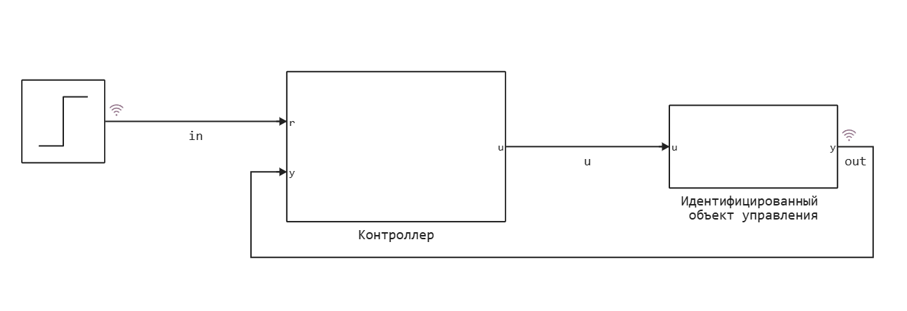
Fuzzy PID controller control system
Let's return to modeling a control system with a fuzzy controller. We have obtained a model of the control object from experimental data.
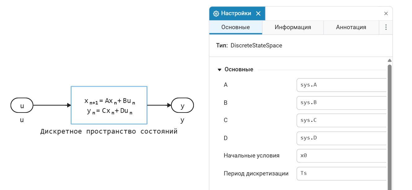
The identification result will be used in the Discrete State Space block to model the control object.
It remains to add the controller to the control system circuit. This example uses the following fuzzy logic controller structure:
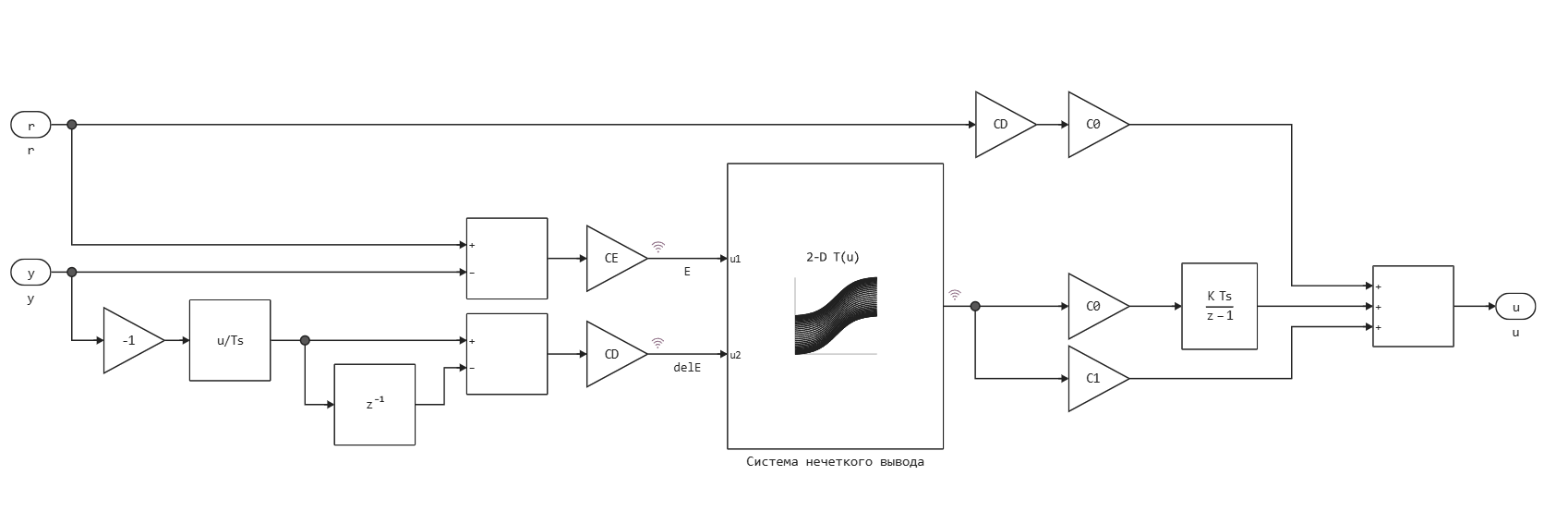
Normalized error values are received at the input of the fuzzy output system and the derived error . The input values are normalized using scaling factors. and so that they are in the range [-1,1].
The fuzzy output system outputs a result in the range [-1, 1], which is scaled by coefficients and .
CE = 10;
CD = 4.9829;
C0 = 2.5179;
C1 = 1.8103;
The fuzzy inference system is represented as a block of a Lookup table. The process of forming the response surface for this table is shown below:
fis = @sugfis function FCtrl(E, delE)::U
    E := begin
        domain = -10.0:10.0
        N = GaussianMF(-10.0, 7.0)
        P = GaussianMF(10.0, 7.0)
    end

    delE := begin
        domain = -10.0:10.0
        N = GaussianMF(-10.0, 7.0)
        P = GaussianMF(10.0, 7.0)
    end

    U := begin
        domain = -20.0:20.0
        Min = -20.0
        Zero = 0.0
        Max  = 20.0
    end

   # Working rules
   E == N  && delE == N  -->  U == Min
   E == N  && delE == P  -->  U == Zero
   E == P  && delE == N  -->  U == Zero
   E == P  && delE == P  -->  U == Max

end;
plot(fis, :E, ylabel="Accessory function", w = 2)
plot(fis, :delE, ylabel="Accessory function", w = 2)
Let's create a response surface in order to place it in the Lookup table block.
errBrkpts = -10.0:0.5:10.0
rateBrkpts = -10.0:0.5:10.0
LookUpTableData = zeros(length(errBrkpts), length(rateBrkpts))
i = 0;
for e in errBrkpts
    i = i+1
    j = 0;
    for de in rateBrkpts
        j = j+1
        LookUpTableData[i, j] = fis([e, de])[:U]
    end
end
surface(errBrkpts, rateBrkpts, LookUpTableData, xlabel="ΔE", ylabel="E", zlabel="U", title="Response surface", camera=(30, 30))
Let's run the control system model and check the operation of the regulator.
if "Fuzzycontroller" in [m.name for m in engee.get_all_models()]
    m = engee.open( "Fuzzycontroller" ) # loading the model
else
    m = engee.load( "Fuzzycontroller.engee" )
end
fuzzyresults = engee.run(m, verbose=true)
fuzzydataout = collect(fuzzyresults["out"]);
fuzzydatain = collect(fuzzyresults["in"]);
In the graphs, we see the response of the control system to the stepwise impact.
plot(fuzzydataout.time, fuzzydataout.value, titel = "Fuzzy PID controller control system", label="exit")
plot!(fuzzydatain.time, fuzzydatain.value, label="entrance")
Conclusion
As a result, we got a working control system with a fuzzy PID controller. The model of the control object was not known in advance, but was obtained by identification based on experimental data.