gr()
engee.open("pid_manual_tuning.engee")
using DataFrames, Statistics
all_runs = DataFrame[];
colors = [1, "skyblue", "lightblue", "powderblue", "lightblue1"];

StopTime = 30 # @param {type:"slider",min:0,max:100,step:1}

P_max = 6.0 # @param {type:"number",placeholder:"1.0"}
I_max = 1.0 # @param {type:"number",placeholder:"1.0"}
D_max = 1.0 # @param {type:"number",placeholder:"1.0"}

P = 0.09 # @param {type:"slider",min:0,max:1,step:0.01}
I = 0.91 # @param {type:"slider",min:0,max:1,step:0.01}
D = 0 # @param {type:"slider",min:0,max:1,step:0.01}

engee.set_param!("pid_manual_tuning/PID controller", "P"=>P*P_max, "I"=>I*I_max, "D"=>D*D_max)
engee.set_param!("pid_manual_tuning", "StopTime"=>StopTime)

# Run the model and get the results.
data = engee.run("pid_manual_tuning")
x = collect(data["x"])
y = collect(data["y"])

# Delete the last item if the list is full.
pushfirst!(all_runs, y)
if length(all_runs) > 5 pop!(all_runs); end;

# Analysis of the last transition process
if length(all_runs) > 0
    last_run = all_runs[1]
    time_data = last_run.time
    value_data = last_run.value
    
    # We determine the steady-state value (the last 10% of the data)
    steady_state_idx = Int.(collect((round(0.9 * length(value_data)):length(value_data))))
    steady_state_value = mean(value_data[steady_state_idx])
    
    # Defining the initial value
    initial_value = value_data[1]
    
    # Target value (we take it from the task)
    target_value = x.value[end]  # assuming that x is the assignment
    
    # We find the maximum deviation (overshoot)
    max_overshoot = maximum(value_data)
    overshoot_percentage = abs((max_overshoot - steady_state_value) / (target_value - initial_value)) * 100
    
    # Installation time (5%)
    tolerance = 0.05 * abs(target_value - initial_value)
    settling_time = nothing
    
    for i in length(value_data):-1:1
        if abs(value_data[i] - steady_state_value) > tolerance
            settling_time = time_data[i]
            break
        end
    end
    
    # Rise time (10%-90%)
    rise_time_10 = nothing
    rise_time_90 = nothing
    
    threshold_10 = initial_value + 0.1 * (steady_state_value - initial_value)
    threshold_90 = initial_value + 0.9 * (steady_state_value - initial_value)
    
    for i in 1:length(value_data)
        if value_data[i] >= threshold_10 && rise_time_10 === nothing
            rise_time_10 = time_data[i]
        end
        if value_data[i] >= threshold_90 && rise_time_90 === nothing
            rise_time_90 = time_data[i]
            break
        end
    end
    
    rise_time = rise_time_90 - rise_time_10
    
    # We display the results of the analysis
    println("═"^50)
    println("ANALYSIS OF THE TRANSITION PROCESS")
    println("═"^50)
    println("Steady-state value: $(round(steady_state_value, digits=3))")
    println("Overshoot: $(round(overshoot_percentage, digits=1))%")
    
    if settling_time !== nothing
        println("Setup time (5%): $(round(setting_time, digits=2)) s")
    else
        println("Setup time: the process has not been established")
    end
    
    if rise_time !== nothing && rise_time_10 !== nothing
        println("Rise time (10%-90%): $(round(rise_time, digits=2)) s")
    end
    
    # Static error (if any)
    static_error = abs(target_value - steady_state_value)
    if static_error > 1e-6
        println("Static error: $(round(static_error, digits=4))")
    else
        println("Static error: missing")
    end
    
    # Number of fluctuations
    peaks = 0
    for i in 2:length(value_data)-1
        if value_data[i] > value_data[i-1] && value_data[i] > value_data[i+1] && 
           value_data[i] > steady_state_value
            peaks += 1
        end
    end
    println("Number of fluctuations: $peaks")
    
    println("═"^50)
end

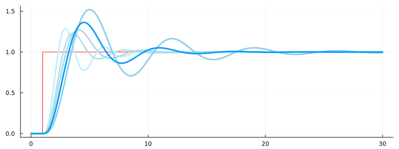
# Output the graphs
plot(x.time, x.value, c=:red, lw=1, size=(800,300), leg=false)
for i in length(all_runs):-1:1
    plot!(all_runs[i].time, all_runs[i].value, c=colors[i], lw=3)
end
plot!()