Simulation of pipeline pressure control using a fuzzy regulator
This example demonstrates the simulation of pressure control in a pipeline using a fuzzy regulator.
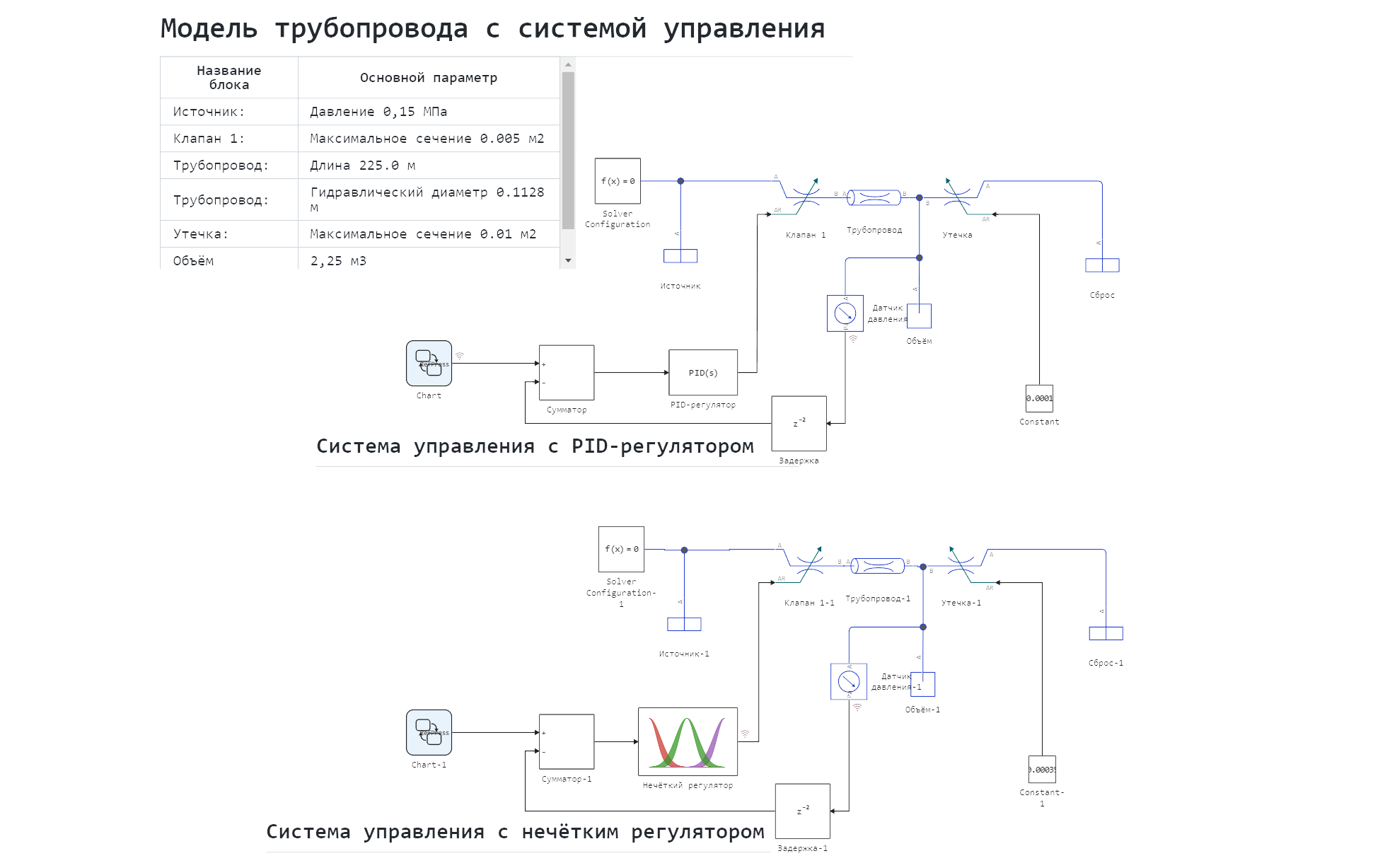
The model file contains two hydraulic circuits with control systems. The upper circuit is controlled by a PID controller, its description can be found in the Community.: Simulation of pressure control in трубопроводе and Pipeline pressure control. The setpoint signal in both circuits is represented by a block
Chart
Нижняя схема имеет аналогичные параметры физических блоков.
Схема модели:
Нечёткий регулятор описан с помощью блока Engee Function. Он позволяет использовать код на языке программирования Julia. Подробнее о работе с Engee Function можно узнать в соответствующей статье документации.
Чтобы создать нечёткий регулятор воспользуемся библиотекой языка программирования Julia, которая называется FuzzyLogic. Для её установки в Engee требуется выполнить следующую кодовую ячейку:
Pkg.add(["FuzzyLogic"])
Pkg.add("FuzzyLogic")
Запускаем установленную библиотеку FuzzyLogic и библиотеку для построения графиков Plots.
using FuzzyLogic
using Plots
В кодовой ячейке ниже осуществляется построение системы нечёткого вывода Мамдани (Mamdani fuzzy inference system) с помощью макроса @mamfis. Построение такой системы включает в себя определение функций принадлежности (Membership functions). Объявляется функция tipper, которая принимает один аргумент delta_p. Эта переменная будет представляет собой входные данные, которые поступают с сумматора, вычисляющего разность между заданным и измеренным давлением.
Функции принадлежности для диапазонов разностей давлений и выходных сигналов площади сечения клапана включают в себя:
- гауссовскую функцию принадлежности
GaussianMF(x, y)- где x - среднее значение, определяющее центр распраделения, а y - стандартное отклонение - треугольную функцию принадлежности
TriangularMF(x, y, z), где x - левый угол треугольника, z - правый, а y - пик треугольника - трапециевидную функцию принадлежности
TrapezoidalMF(x, y, z, k), где x - левый нижний угол трапеции, k - правый нижний угол, y и z - левый верхний и правый верхний углы соответственно
В переменной domain определяются диапазоны в которых будут определены функции принадлежности.
Далее определяются правила нечёткой логики, которые связывают входные и выходные переменные. Например:
Если delta_p очень высокое, то control_signal будет полностью открытым.
Если delta_p высокое, то control_signal будет частично открытым.
И так далее для остальных условий.
fis = @mamfis function tipper(delta_p)::control_signal
    delta_p := begin
        domain = -50000.0:50000.0
        very_high = GaussianMF(17000.0, 3000.0)  # Very high pressure
        high = GaussianMF(15000.0, 4120.0)       # High pressure
        moderate = GaussianMF(-6000.0, 3000.0)       # Normal pressure
        low = GaussianMF(-15000.0, 3000.0)       # Low pressure
        very_low = GaussianMF(-30000.0, 3000.0)  # Very low pressure
    end

    control_signal := begin
        domain = 0.0:0.005
        fully_closed = TriangularMF(0.00000000001, 0.00000001, 0.000001)  # Fully closed flap
        partially_closed = TriangularMF(0.0000009, 0.000005, 0.00001)  # Partially closed flap
        neutral = TriangularMF(0.00001, 0.00002, 0.0003)  # Neutral position (half open)
        partially_open = TrapezoidalMF(0.0003, 0.0009, 0.003, 0.0044)  # Partially open flap
        fully_open = TriangularMF(0.004, 0.0047, 0.005)  # Fully open flap
    end

    # Working rules
    delta_p == very_high --> control_signal == fully_open
    delta_p == high --> control_signal == partially_open
    delta_p == moderate --> control_signal == neutral
    delta_p == low --> control_signal == partially_closed
    delta_p == very_low --> control_signal == fully_closed
end
Вывод на график функций принадлежности для входных данных:
plot(fis, :delta_p)
Вывод на график функций принадлежности для выходных данных данных:
plot(fis, :control_signal)
Для того чтобы реализовать данную систему нечёткого вывода в виде системы управления, необходимо сгенерировать из неё функцию, не зависящую от библиотеки и определяемую только базовыми конструкциями языка Julia. Для этого можно использовать функцию compilefis(fis), где аргумент fis это система нечёткого вывода, определённая ранее и записанная в переменную. Результат кодогенерации с помощью данной функции записывается в переменную asd:
asd = compilefis(fis)
The result recorded in the asd variable is rewritten into a code cell.:
function tipper(delta_p)
    very_high = exp(-((delta_p - 17000.0) ^ 2) / 1.8e7)
    high = exp(-((delta_p - 15000.0) ^ 2) / 3.39488e7)
    moderate = exp(-((delta_p - -6000.0) ^ 2) / 1.8e7)
    low = exp(-((delta_p - -15000.0) ^ 2) / 1.8e7)
    very_low = exp(-((delta_p - -30000.0) ^ 2) / 1.8e7)
    ant1 = very_high
    ant2 = high
    ant3 = moderate
    ant4 = low
    ant5 = very_low
    control_signal_agg = collect(LinRange{Float64}(0.0, 0.005, 101))
    @inbounds for (i, x) = enumerate(control_signal_agg)
            fully_closed = max(min((x - 1.0e-11) / 9.99e-9, (1.0e-6 - x) / 9.9e-7), 0)
            partially_closed = max(min((x - 9.0e-7) / 4.1000000000000006e-6, (1.0e-5 - x) / 5.0e-6), 0)
            neutral = max(min((x - 1.0e-5) / 1.0e-5, (0.0003 - x) / 0.00028), 0)
            partially_open = max(min((x - 0.0003) / 0.0006000000000000001, 1, (0.0044 - x) / 0.0014000000000000002), 0)
            fully_open = max(min((x - 0.004) / 0.0007000000000000001, (0.005 - x) / 0.0002999999999999999), 0)
            control_signal_agg[i] = max(max(max(max(min(ant1, fully_open), min(ant2, partially_open)), min(ant3, neutral)), min(ant4, partially_closed)), min(ant5, fully_closed))
        end
    control_signal = ((2 * sum((mfi * xi for (mfi, xi) = zip(control_signal_agg, LinRange{Float64}(0.0, 0.005, 101)))) - first(control_signal_agg) * 0.0) - last(control_signal_agg) * 0.005) / ((2 * sum(control_signal_agg) - first(control_signal_agg)) - last(control_signal_agg))
    return control_signal
end
By defining the function tipper() describing the fuzzy output system, we can plot the dependence of the output data on the input data. To do this, we determine the vector of pressure values from -50000 to 50,000 Pa, as previously written in the variable domain and we pass it through the function:
x = collect(range(-50000.0,50000.0,10001));
Plotting the response curve of the resulting function:
plot(x, tipper.(x), linewidth=3)
There is a graph of the dependence of the valve opening area on the pressure difference between the setpoint and the signal from the sensor.
The function obtained by code generation can be written to a file. To do this, the asd variable in Expr format is converted to String format for further writing.:
text_function = string(asd)
Writing a function in string format to a file:
f = open("/user/start/examples/controls/liquid_pressure_regulator_fuzzy/liquid_pressure_regulator_fuzzy.jl","w") # creating a file
write(f, text_function) # writing to a file
close(f) # closing the file
The resulting file, in .jl format, with the function tipper(), we put it in the block Engee Function and we perform using the function include(). To do this, go to the block parameters, click on the "Look under the mask" button, select the "Main" tab and click "Edit source code", enter in the window that opens:
struct Block <: AbstractCausalComponent; end

function (c::Block)(t::Real, delta_p)
    include("liquid_pressure_regulator_fuzzy.jl")
    return control_signal
end
Next, the model is launched and data is displayed on graphs.
Defining a function to load and run the model:
function start_model_engee()
    try
        engee.close("liquid_pressure_regulator_fuzzy", force=true) # closing the model
        catch err # if there is no model to close and engee.close() is not executed, it will be loaded after catch.
            m = engee.load("$(@__DIR__)/liquid_pressure_regulator_fuzzy.engee") # loading the model
        end;

    try
        engee.run(m) # launching the model
        catch err # if the model is not loaded and engee.run() is not executed, the bottom two lines after catch will be executed.
            m = engee.load("$(@__DIR__)/liquid_pressure_regulator_fuzzy.engee") # loading the model
            engee.run(m) # launching the model
        end
end
Running the simulation
try
    start_model_engee() # running the simulation using the special function implemented above
    catch err
    end;
Extracting data from the simout variable and writing it to variables:
sleep(5)
result = simout;
res = collect(result)
Recording of signals from the setpoint sensor and pressure sensors of both circuits into variables:
PID_regulator = collect(res[1])
Fuzzy control = collect(res[3])
Sensor signal_= collect(res[4]);
Visualization of simulation results
plot(PID_регулятор[:,1], PID_регулятор[:,2], linewidth=3, label="The PID controller")
plot!(Нечёткий_регулятор[:,1], Нечёткий_регулятор[:,2], linewidth=3, label="Fuzzy controller")
plot!(Сигнал_задатчика[:,1], Сигнал_задатчика[:,2], linewidth=3, label="Setter signal")
Analyzing the graph, you can see that, unlike the PID controller, the fuzzy controller has significantly less overshoot, as well as a shorter duration of the transient process. But the fuzzy controller also has a disadvantage, its signal can often be shifted from the setpoint signal by a certain amount, but this can be corrected by more precise adjustment of the membership functions and decision rules.
Conclusion:
In this example, we demonstrated the simulation of two physical objects with different variants of automatic control systems, in particular, with a PID controller and a fuzzy controller. A fuzzy inference system was built, which was then transformed into a function suitable for embedding in the Engee Function block. The result is a fuzzy controller, which is not inferior in its characteristics to a PID controller.