Adaptive binarization
Binarization is one of the key steps in image preprocessing, especially in character recognition (OCR), document analysis, and computer vision tasks. It converts a grayscale image to black and white, highlighting foreground objects against the background. However, standard global threshold methods such as the Otsu algorithm often fail in the presence of uneven lighting, gradient shadows, or complex backgrounds. In such cases, local (adaptive) methods that calculate the threshold for each pixel based on the neighborhood turn out to be much more efficient.
In this example using packages Images, ImageBinarization, ImageFiltering and ImageMorphology The full image processing pipeline is demonstrated, starting with the synthesis of a test image with uneven lighting and ending with the preparation of a binary image for OCR. The main focus is on comparing global Ots binarization and two adaptive methods based on local mean and Gaussian weighting. The following shows the application of morphological operations (opening and closing) to eliminate noise, the construction of the skeleton of objects and the final inversion, convenient for OCR. The example clearly illustrates the advantages of adaptive approaches and shows how their combination with morphology allows you to get high-quality results even in images with difficult lighting.
# Pkg.add(["ImageBinarization", "ImageMorphology"]
using Images, TestImages, ImageFiltering, ImageBinarization, ImageMorphology
1. Image generation with uneven lighting
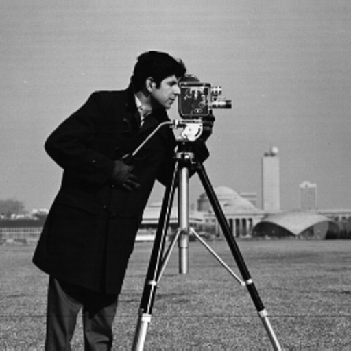
The original cameraman image is distorted by a gradient shadow (linearly increasing from the corners to the center), simulating real shooting conditions. Such coverage makes it difficult to choose a single global threshold.
img = testimage("cameraman")
h, w = size(img)
shadow = [Gray(0.3 + 0.7 * (j/w + i/h)/2) for i in 1:h, j in 1:w]
img_uneven = img .* shadow

display(img)
println("The original")

display(img_uneven)
println("With uneven lighting")

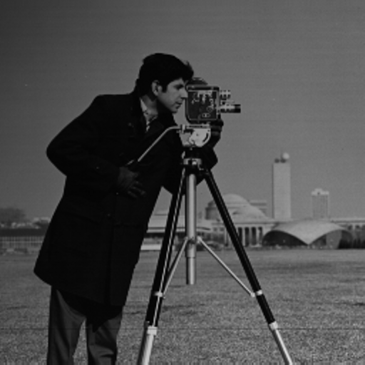
img_gray = Gray.(img_uneven)
display(img_gray)
println("Gradations of gray")
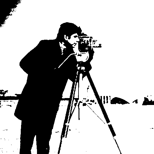
2. Global Binarization (Otsu)
Applying the Otsu method to the entire image leads to significant losses: dark areas turn into a solid background, while light areas, on the contrary, may be mistakenly attributed to the foreground. The result shows that the global threshold is unsuitable for this case.
img_otsu = binarize(img_gray, Otsu())
display(img_otsu)
println("Global Otsu")
3. Adaptive binarization with local mean
A function has been implemented that calculates for each pixel the average value in a sliding block of a given size. (11×11, 21×21, 51×51). The threshold is defined as the "mean – constant C". If the block size (11) is small, excessive detail and noise appear; if it is too large (51), the method approaches the global one. The optimal size (21) gives a good separation of objects without much noise.
function adaptive_threshold_mean(img, block_size; C=0.0)
    h, w = size(img)
    result = similar(img, Bool)
    half_block = div(block_size, 2)
    for i in 1:h
        for j in 1:w
            i1 = max(1, i - half_block)
            i2 = min(h, i + half_block)
            j1 = max(1, j - half_block)
            j2 = min(w, j + half_block)
            block_mean = mean(img[i1:i2, j1:j2])
            result[i, j] = img[i, j] > (block_mean - C)
        end
    end
    return result
end

for bs in [11, 21, 51]
    img_adaptive_mean = adaptive_threshold_mean(img_gray, bs, C=0.05)
    display(Gray.(img_adaptive_mean))
    println("Adaptive Mean, block $(bs)x$(bs)")
end
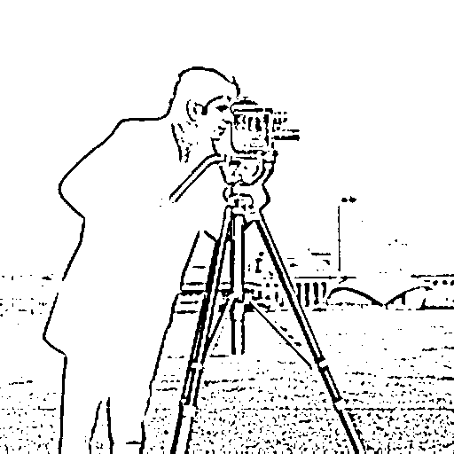


4. Adaptive binarization with Gaussian weighting
Instead of uniform averaging, the Gaussian kernel is used, which gives more weight to the central pixels of the block. This approach is more resistant to emissions and preserves the boundaries of objects better. Using the example of the 21x21 block, you can see that the result is cleaner than using a simple average.
function adaptive_threshold_gaussian(img, block_size; C=0.0, sigma=0.0)
    h, w = size(img)
    result = similar(img, Bool)
    half_block = div(block_size, 2)
    if sigma == 0
        sigma = 0.3 * ((block_size - 1) * 0.5 - 1) + 0.8
    end
    x = -half_block:half_block
    kernel_1d = [exp(-(i^2)/(2*sigma^2)) for i in x]
    kernel_1d = kernel_1d / sum(kernel_1d)
    kernel = kernel_1d * kernel_1d'
    for i in 1:h
        for j in 1:w
            i1 = max(1, i - half_block)
            i2 = min(h, i + half_block)
            j1 = max(1, j - half_block)
            j2 = min(w, j + half_block)
            block = img[i1:i2, j1:j2]
            ki1 = half_block - (i - i1) + 1
            ki2 = half_block + (i2 - i) + 1
            kj1 = half_block - (j - j1) + 1
            kj2 = half_block + (j2 - j) + 1
            k = kernel[ki1:ki2, kj1:kj2]
            k = k / sum(k)
            weighted_mean = sum(block .* k)
            result[i, j] = img[i, j] > (weighted_mean - C)
        end
    end
    return result
end

img_adaptive_gauss = adaptive_threshold_gaussian(img_gray, 21, C=0.05)
display(Gray.(img_adaptive_gauss))
println("Adaptive Gaussian, block 21x21")

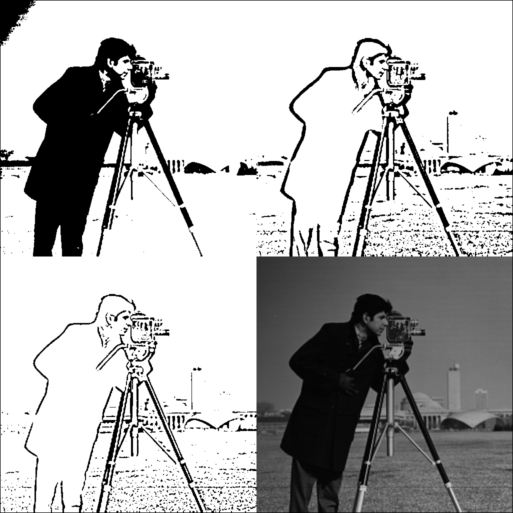
5. Comparative visualization
A grid is created where the results of Otsu, adaptive mean, adaptive Gaussian, and the original grayscale image are presented simultaneously. The difference between the methods becomes obvious: adaptive methods successfully compensate for the lighting gradient, while the Gaussian version provides the most balanced binary representation.
function create_comparison_grid(images, titles)
    n = length(images)
    h, w = size(images[1])
    grid_h = h * 2
    grid_w = w * 2
    grid = fill(Gray(0.5), grid_h, grid_w)
    positions = [(1:h, 1:w), (1:h, w+1:2*w), (h+1:2*h, 1:w), (h+1:2*h, w+1:2*w)]
    for (i, (img, pos)) in enumerate(zip(images, positions))
        if i <= n
            grid[pos...] = Gray.(img)
        end
    end
    return grid
end

comparison = create_comparison_grid(
    [img_otsu, adaptive_threshold_mean(img_gray, 21, C=0.05), img_adaptive_gauss, img_gray],
    ["Otsu", "Adaptive Mean", "Adaptive Gaussian", "Original"]
)
display(comparison)
println("Comparison: Otsu | Mean | Gaussian | Original")
6. Morphological processing
For the best result (adaptive Gauss), the opening and closing operations are applied. Opening removes small noise points, and closing fills small gaps in the contours of objects. This is an important step before further analysis of the form.
img_binary = Gray.(img_adaptive_gauss)
img_opened = opening(img_binary)
display(img_opened)
println("After opening")
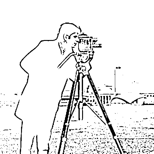
img_closed = closing(img_opened)
display(img_closed)
println("After closing")
7. Skeletonization
The algorithm of skeletonization is implemented (search for the "skeleton" – the centerlines of objects). In a binary image, after morphology, the skeleton allows you to highlight the topological structure of the shapes, which can be used for recognition or measurement.
function skeletonize(img)
    img_bool = Bool.(img)
    skeleton = copy(img_bool)
    changed = true
    while changed
        changed = false
        to_remove = []
        for i in 2:size(skeleton, 1)-1
            for j in 2:size(skeleton, 2)-1
                if !skeleton[i, j]
                    continue
                end
                p = [
                    skeleton[i-1, j], skeleton[i-1, j+1], skeleton[i, j+1],
                    skeleton[i+1, j+1], skeleton[i+1, j], skeleton[i+1, j-1],
                    skeleton[i, j-1], skeleton[i-1, j-1]
                ]
                nonzero = sum(p)
                if nonzero < 2 || nonzero > 6
                    continue
                end
                transitions = sum([p[k] == 0 && p[mod1(k+1, 8)] == 1 for k in 1:8])
                if transitions != 1
                    continue
                end
                if p[1] * p[3] * p[5] == 0 && p[3] * p[5] * p[7] == 0
                    push!(to_remove, (i, j))
                    changed = true
                end
            end
        end
        for (i, j) in to_remove
            skeleton[i, j] = false
        end
        to_remove = []
        for i in 2:size(skeleton, 1)-1
            for j in 2:size(skeleton, 2)-1
                if !skeleton[i, j]
                    continue
                end
                p = [
                    skeleton[i-1, j], skeleton[i-1, j+1], skeleton[i, j+1],
                    skeleton[i+1, j+1], skeleton[i+1, j], skeleton[i+1, j-1],
                    skeleton[i, j-1], skeleton[i-1, j-1]
                ]
                nonzero = sum(p)
                if nonzero < 2 || nonzero > 6
                    continue
                end
                transitions = sum([p[k] == 0 && p[mod1(k+1, 8)] == 1 for k in 1:8])
                if transitions != 1
                    continue
                end
                if p[1] * p[3] * p[7] == 0 && p[1] * p[5] * p[7] == 0
                    push!(to_remove, (i, j))
                    changed = true
                end
            end
        end
        for (i, j) in to_remove
            skeleton[i, j] = false
        end
    end
    return skeleton
end

img_skeleton = skeletonize(img_closed)
display(Gray.(img_skeleton))
println("Skeleton")
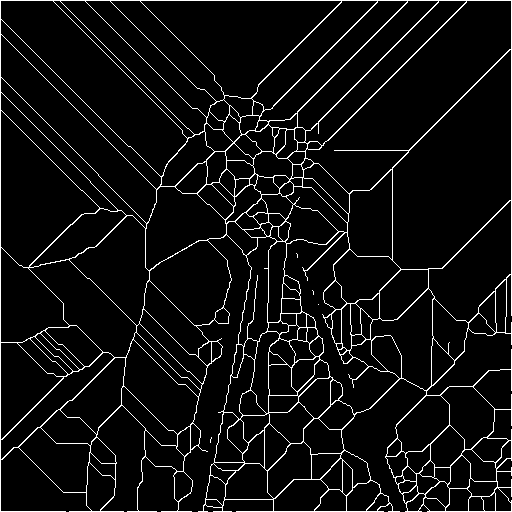
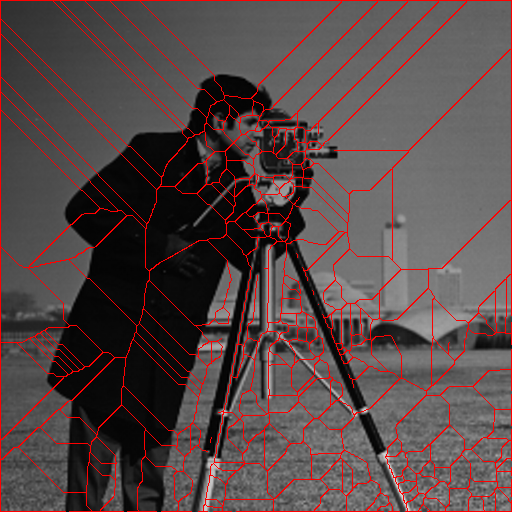
img_overlay = RGB.(img_gray)
skeleton_coords = findall(img_skeleton)
for coord in skeleton_coords
    img_overlay[coord] = RGB(1, 0, 0)
end
display(img_overlay)
println("Skeleton overlay (red)")
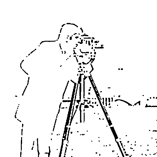
img_for_ocr = Gray.(.! Bool.(img_closed))
display(Gray.(img_for_ocr))
println("For OCR (inversion)")

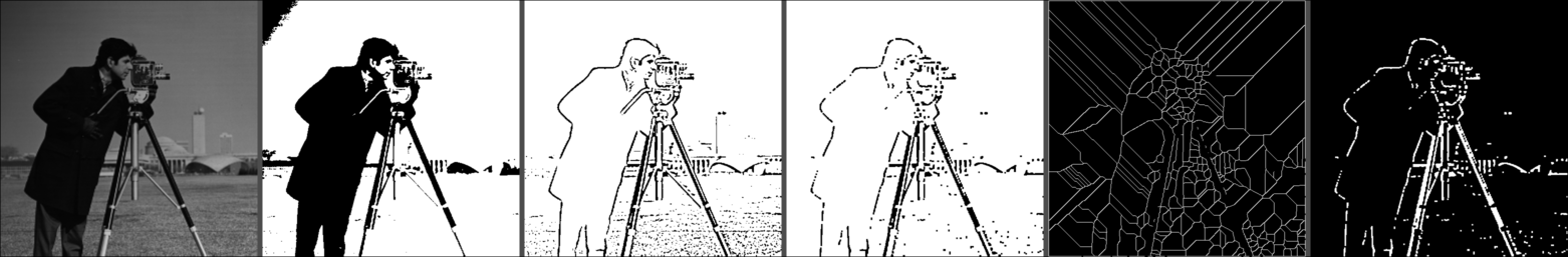
8. Preparation for OCR
The final image is inverted (black characters on a white background) – the standard format for most OCR systems. Visualization of the entire pipeline (from the original grayscale to ready for OCR) clearly demonstrates the effect of each step.
function create_pipeline_visualization(images, titles)
    n = length(images)
    h, w = size(images[1])
    result = fill(Gray(0.3), h, w * n + (n-1) * 10)
    for (i, img) in enumerate(images)
        start_col = (i-1) * (w + 10) + 1
        end_col = start_col + w - 1
        result[:, start_col:end_col] = Gray.(img)
    end
    return result
end

pipeline = create_pipeline_visualization(
    [img_gray, img_otsu, img_adaptive_gauss, img_closed, img_skeleton, img_for_ocr],
    ["Gray", "Otsu", "Adaptive", "Denoised", "Skeleton", "OCR Ready"]
)
display(pipeline)
println("The complete pipeline")
Conclusion
In the course of working with the example, we studied and saw in practice:
- Limitations of global binarization in uneven lighting.
- Advantages of adaptive methods, especially Gaussian weighting, which allows taking into account local contrast and suppressing artifacts.
- The effect of the size of the local block on the result: too small a block increases noise, too large reduces adaptability.
- The need for morphological post-processing to eliminate noise and restore the integrity of objects.
- The possibility of skeletonization for shape and topology analysis.
- Building a complete pipeline suitable for practical OCR tasks.
The example showed that the correct choice of the binarization method and subsequent processing can significantly improve the quality of object selection, even in complex images. The knowledge gained can be directly applied in the development of text recognition systems, document analysis, and other applications where resistance to uneven lighting is important.