Working with pixel matrices

Images using the package Images they are multidimensional arrays — in fact, matrices, where each element contains a color value (for example, RGBThis approach makes it easy to manipulate pixels using standard array operations: indexing, slices, piecemeal calculations, etc.

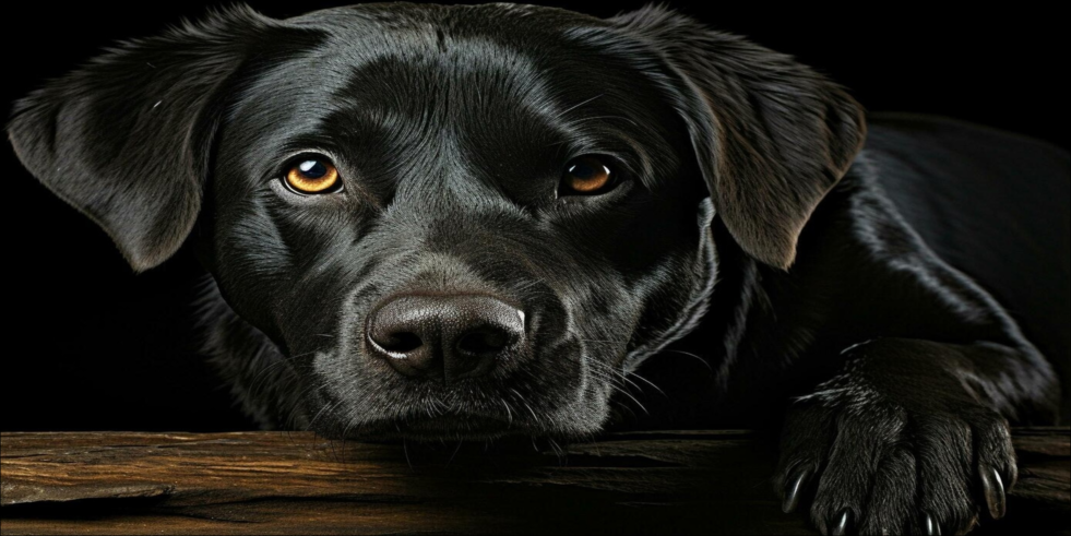
In this example, we solve the following problem: upload an arbitrary image, divide it into equal vertical stripes, then assemble the stripes with odd numbers and the stripes with even numbers separately, forming two new images. Finally, we display them side by side for visual comparison.

This example clearly demonstrates:

• how to upload and display an image;
• how to get its dimensions;
• how to calculate the number of lanes and their width, taking into account the remainder;
• how to create new arrays (images) and fill them with pixels from the original;
• how to use loops and conditional operators to process each pixel.

Thus, we learn the basic techniques of working with images as with matrices, which is the foundation for more complex computer vision and graphics processing algorithms, the code is written using packages. Images, FileIO and ImageShow.

Step 1. Upload the image and get its characteristics

In this block, we:

• Uploading an image from a file IMG.jpg using the function load from the package FileIO. The result is saved to a variable original_img. Now original_img is a multidimensional array (matrix), each element of which contains a pixel color in the format RGB (or shades of gray if the image is black and white).
• We display the image on the screen using display. This is possible thanks to the package ImageShow, which provides the display of graphical objects.
• We get the dimensions of the image: height (height, number of rows) and width (width, number of columns). Function size returns a tuple, which we decompress into two variables.
• Print the received values to the console using println. This allows you to make sure that the image has been uploaded correctly and find out its resolution.

Important: for working with color images, the package Images it automatically represents them as a matrix of elements of the type RGB (or RGB4). Each such element contains fields r, g, b (red, green, blue) with values from 0 to 1. Thus, we can access individual pixels, for example original_img[100, 200] will give the color of the pixel in row 100, column 200.

At this stage, we have prepared the initial data for further processing.

Step 2. Define the parameters of the bands

Here we prepare everything necessary to divide the image into vertical stripes.:

• n_stripes = min(height, width)
  The number of stripes is selected equal to the minimum size of the image. This ensures that there will be no more stripes than rows or columns, and each stripe will have sufficient width (in pixels) for visibility.

• base_width = div(width, n_stripes)
  We calculate the base bandwidth as an integer division of the total width by the number of lanes. Since the width may not be completely divisible, some of the stripes will be one pixel wider.

• remainder = width % n_stripes
  The remainder of the division is how many stripes an additional pixel will have.

• widths = [i <= remainder ? base_width + 1 : base_width for i in 1:n_stripes]
  Creating an array widths, where for each lane i its width is specified. First remainder stripes get a width of base_width + 1, the rest — base_width. Thus, all the stripes have almost the same width, differing by a maximum of 1 pixel, which allows them to evenly cover the entire width of the image.

• max_width = maximum(widths)
  Find the maximum width among all the lanes. This will be required later when we create images for storing stripes: each stripe will be represented by a rectangle of the same height (equal to the height of the original image) and the same width. max_width so that they can be easily glued together. The narrower stripes will be complemented by black pixels on the right.

• odd_stripes = [] and even_stripes = []
  Initialize two empty arrays to store the strips themselves: in odd_stripes we will add the stripes with odd numbers, in even_stripes — with even numbers.

• start_col = 1
  Counter variable, which will indicate the beginning of the next stripe in the original image during the next pass.

At this stage, we have fully prepared the data for the strip extraction cycle: we know how many of them there are, how wide they are, and we are ready to divide them by parity.

Step 3. Extract the stripes from the original image

In this cycle, we sequentially go through all the lanes from left to right and perform the following actions:

• Defining the boundaries of the lane:
  Using the current value start_col (left edge) and width w, we calculate end_col — the right edge of the lane. This way we know which column range of the original image corresponds to the i-th band.

• Cut out the rectangle:
  stripe_rect = original_img[:, start_col:end_col] — we take all the lines (:) and the necessary columns. It turns out a matrix of size height × w, containing the pixels of the given strip.

• Creating a standardized rectangle:
  stripe_img = similar(original_img, height, max_width) creates a new matrix (image) of the same type as the original one, but in size height × max_width. This is necessary so that all the stripes have the same width — then they will be easy to glue into the final images. img1 and img2.
  Then fill!(stripe_img, RGB(0,0,0)) fills this rectangle with black (all components are 0).

• Copy the pixels of the strip:
  stripe_img[:, 1:w] = stripe_rect — insert the cut-out fragment into the left part of the created rectangle. If the streak was narrower than max_width, black pixels will remain on the right (background).

• Sort by parity:
  Using isodd(i) we check the lane number. Add the odd stripes to the array odd_stripes, even — numbered - in even_stripes. This is how we divide the stripes into two groups to create two separate images later.

• Shifting the beginning:
  start_col += w — we increase the counter by the width of the newly processed strip, so that in the next iteration we can start from the place where the current one ended.

As a result, after the loop, we have two arrays, each of which contains a set of matrices (strips) of the same size. height × max_width, moreover, all pixels from the source image are distributed along these stripes in accordance with their order.

Step 4. We form two images from bands of different parity

At this stage, we combine the individual stripes into two integral images.:

• Creating canvases:
  img1 and img2 created using similar, which guarantees the same pixel type as the original image. Their height is equal to the height of the original (height), and the width is calculated as max_width (maximum bandwidth) multiplied by the number of lanes of the corresponding group.
  For example, if we have 10 lanes, then in odd_stripes there will be 5 stripes (odd), which means the width is img1 = max_width * 5.
  Then both images are filled with black (RGB(0,0,0)) — this will be the background on which we will overlay the pixels of the stripes.

• Assembling an image from odd stripes:
  Variable col_offset tracks the current position (column) in the final image, starting from 1. In a loop across all stripes from odd_stripes we:

  • determining the actual width of the current lane w (it is equal to max_width since all the stripes have been expanded to this size);
  • insert the strip matrix stripe to the appropriate range of columns img1[:, col_offset:col_offset+w-1];

• zoom in col_offset on w moving on to the location for the next lane.

• Assembling an image from even stripes:
  A similar cycle is performed for even_stripes, forming img2.

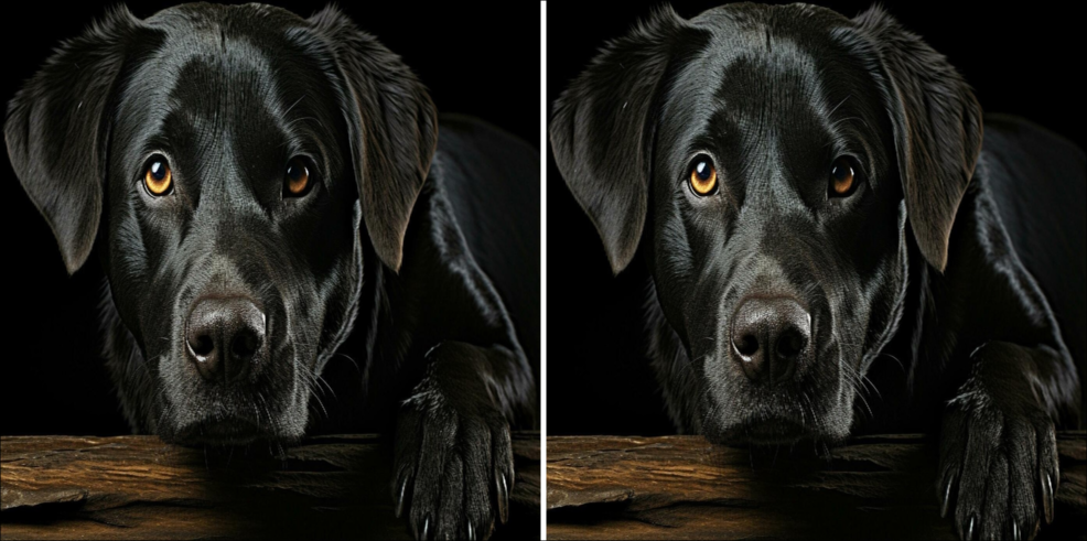
As a result, we get two images, each of which represents horizontally glued strips of the original image.:

• img1 contains bands 1, 3, 5, ... (odd);
• img2 contains bands 2, 4, 6, ... (even).

Please note: since all the stripes have been reduced to a single width max_width, in img1 and img2 there are no gaps between the fragments — they are located close together. Black areas to the right of the narrower stripes (if the original width of the stripe was smaller max_width) are preserved, so there may be vertical black stripes at the joints — this is an artifact of alignment, but it does not interfere with further comparison.

Step 5. Combine the two images for comparison and output the result

At this final stage, we:

• We get the dimensions of the generated images:
  h1, w1 = size(img1) and h2, w2 = size(img2). Both images have the same height (height the original image), but the width may vary if the number of odd and even stripes is different (for example, if the total number of stripes is odd). In our example, both turned out to be 980 pixels each, because the original width is 1960, the number of stripes is 980, and there are equally odd/even ones.

• Creating a shared canvas side_by_side:
  max_h = max(h1, h2) — select the maximum height (they are equal, but the code is universal).
  side_by_side = similar(img1, max_h, w1 + w2 + 10) — create a canvas image of the same type as img1, height max_h and a width equal to the sum of the widths of the two images plus 10 pixels of the gap.
  fill!(side_by_side, RGB(1,1,1)) — fill the canvas with white color (all components are equal to 1). The white background creates a visual separator between the two images.

• We place images on the canvas:
  side_by_side[1:h1, 1:w1] = img1 — copy it img1 to the left side of the canvas (rows 1:h1, columns 1:w1).
  side_by_side[1:h2, w1+11:w1+w2+10] = img2 — insert img2 on the right, starting from the position w1+11 (we leave 10 pixels of white space after img1, plus one pixel of indexing — therefore +11). The range of columns captures exactly w2 columns.

• Displaying the result:
  display(side_by_side) It shows the final composite image, where the stripes with odd numbers are on the left and the stripes with even numbers are on the right. The white stripe between them makes it easy to visually separate the pictures.

• We output the dimensions to the console:
  println tells us the exact dimensions of the received images. This is useful for checking and understanding how the original image was transformed.

Conclusion

We have come all the way from uploading an image to visualizing the result of its unusual "cutting". This example clearly shows how to work with images using them as ordinary matrices: extract fragments, create new arrays, fill them with pixels and glue them together. This approach underlies many computer vision and graphics processing tasks, from simple crop to complex filters and transformations.

Interesting fact: Despite the fact that we divided the original image into two groups of stripes (odd and even), visually the new images look identical, this is due to the original symmetry of the image.