Key point detection and matching

In modern computer vision, the key task is to find geometric correspondences between images. Whether it's creating panoramas, tracking an object's movement, or reconstructing a 3D scene from photographs, the whole process is based on detecting unique points and matching them.

The presented code is an instructional but functional implementation of the classic feature detection and matching pipeline. Unlike using a "black box" of ready-made libraries (for example, OpenCV), this example in Julia demonstrates manual programming. It not only shows how to apply algorithms, but also reveals the mathematical essence and algorithmic details of each stage.

Next, connect the libraries:

Images: A basic package for working with images, providing data types and basic input/output functions.
TestImages: A library of standard test images.
ImageFeatures: Contains ready-made algorithms for detecting key points, although this example implements its own version of the Harris detector.
ImageDraw: Designed for rendering graphical primitives, whose functions in the code are replaced by manual implementation for educational purposes.
ImageFiltering: Provides the filtering and convolution tools needed to calculate gradients by the Sobel operator.
CoordinateTransformations: A framework for describing and composing geometric transformations of coordinate space.
Rotations: A specialized package for working with rotation and rotation matrices in computer vision tasks.
StaticArrays: Provides high-performance fixed-size arrays for efficient vector math.
LinearAlgebra: A standard linear algebra library used to solve systems of equations in homography estimation.
Statistics: A standard module for calculating statistical metrics such as the mean and standard deviation of descriptors.

# Pkg.add(["Images", "TestImages", "ImageFeatures", "ImageDraw", "ImageFiltering", "CoordinateTransformations", "Rotations", "StaticArrays"])
using Images, TestImages, CoordinateTransformations, Rotations, StaticArrays, LinearAlgebra, Statistics

Next, we will perform a detailed analysis of the auxiliary rendering functions, both functions implement the classic ** Bresenham algorithms** — effective rasterization methods for geometric primitives using only integer arithmetic.

Function draw_line! The Bresenham algorithm for line drawing. The algorithm builds a line between the points and selecting the pixel closest to the ideal straight line at each step.

The equation of a straight line:

Instead of calculating (which requires division and floating arithmetic), Bresenham uses the error term function, which shows the deviation of the current pixel from the ideal line.

Also, at each step, the algorithm evaluates how much the current point deviates from the ideal straight line. The discrepancy function is updated according to the rules:

Multiplication by 2 (e2 = 2 * err) allows you to avoid working with fractional numbers while maintaining the accuracy of the comparison.

Function draw_circle!: The Midpoint Circle Algorithm. The algorithm builds a circle of radius with a center using eight-way symmetry: if the point if it lies on a circle, then the points symmetrical to it also belong to it:

The equation of a circle:

**The decision parameter evaluates the position of the midpoint between two candidates:

Formulas Solution parameter updates

Parameter It is updated recurrently, without calculating squares at each step.:

These formulas are obtained by decomposition and the exclusion of repetitive calculations.

function draw_line!(img, p1, p2, color)
    x1, y1 = round(Int, p1[1]), round(Int, p1[2])
    x2, y2 = round(Int, p2[1]), round(Int, p2[2])
    dx = abs(x2 - x1)
    dy = abs(y2 - y1)
    sx = x1 < x2 ? 1 : -1
    sy = y1 < y2 ? 1 : -1
    err = dx - dy
    x, y = x1, y1
    while true
        if 1 <= x <= size(img,2) && 1 <= y <= size(img,1)
            img[y, x] = color
        end
        if x == x2 && y == y2
            break
        end
        e2 = 2 * err
        if e2 > -dy
            err -= dy
            x += sx
        end
        if e2 < dx
            err += dx
            y += sy
        end
    end
end

function draw_circle!(img, center, radius, color)
    cx, cy = round(Int, center[1]), round(Int, center[2])
    r = radius
    x = 0
    y = r
    d = 3 - 2r
    while x <= y
        for (dx, dy) in [(x, y), (y, x), (-x, y), (-y, x), (x, -y), (y, -x), (-x, -y), (-y, -x)]
            px = cx + dx
            py = cy + dy
            if 1 <= px <= size(img,2) && 1 <= py <= size(img,1)
                img[py, px] = color
            end
        end
        if d < 0
            d += 4x + 6
        else
            d += 4(x - y) + 10
            y -= 1
        end
        x += 1
    end
end

draw_circle! (generic function with 1 method)

Harris Angle Detector: harris_corners

This function implements the classic Harris-Stevens algorithm (1988)** To detect angles, which are characteristic image points that are resistant to rotations, changes in lighting, and slight geometric distortions.

An angle is a point where the intensity of an image changes significantly in two directions simultaneously. The algorithm analyzes the local window around each pixel and evaluates how "angular" it is.

The matrix of the second moment (Structure Tensor), a matrix is built for each pixel :

Where:

— image gradients along the X and Y axes
Summation is performed along the window around the pixel (in the code, a 3×3 window)

Eigenvalue analysis matrices :

Type of area			Visually
Flat	Small	Small	Homogeneous area
Border	Large	Small	The edge of the object
Angle	Large	A big one	Crossing borders

Instead of calculating eigenvalues (an expensive operation), an approximation is used.:

Where:

— empirical coefficient (usually 0.04–0.06)

Interpretation of the response:

→ Angle (both eigenvalues are large)
→ Border (one large, one small)
→ Flat area (both small)

, Visualization of the detector operation

Исходное изображение → Градиенты → Матрица M → Отклик R → Порог → Локальные максимумы
     [512×512]        [Ix, Iy]     [Sxx,Sxy,Syy]  [R]    [>1% max]   [5×5 окно]

Пример откликов в разных областях:

Область					Тип
Плоская	0.1	0.1	0.0	~0.01	❌
Граница	10.0	0.1	0.5	~−0.4	❌
Угол	10.0	10.0	2.0	~+96	✅

⚙️ Параметры и их влияние

Параметр	Значение по умолчанию	Эффект увеличения	Эффект уменьшения
`k`	0.04	Меньше углов, только самые выраженные	Больше углов, выше чувствительность к шуму
`threshold`	0.01	Только сильные углы (10% от максимума)	Больше углов, включая слабые
Окно сглаживания	3×3	Более устойчиво к шуму	Лучшая локализация, но шумнее
Окно NMS	5×5	Более разреженные точки	Плотнее точки, возможны дубликаты

function harris_corners(img; k=0.04, threshold=0.01)
    img_f = Float64.(img)
    img_f = replace(img_f, NaN => 0.0, Inf => 0.0, -Inf => 0.0)
    Ix = imfilter(img_f, Kernel.sobel()[1])
    Iy = imfilter(img_f, Kernel.sobel()[2])
    Ixx = Ix.^2
    Iyy = Iy.^2
    Ixy = Ix .* Iy
    window = ones(3,3) ./ 9
    Sxx = imfilter(Ixx, window)
    Syy = imfilter(Iyy, window)
    Sxy = imfilter(Ixy, window)
    det = Sxx .* Syy - Sxy.^2
    trace = Sxx + Syy
    response = det - k * trace.^2
    max_resp = maximum(response)
    corners = findall(response .> threshold * max_resp)
    local_max = []
    for c in corners
        i, j = c.I
        val = response[i,j]
        r_min = max(1, i-2)
        r_max = min(size(img,1), i+2)
        c_min = max(1, j-2)
        c_max = min(size(img,2), j+2)
        window_vals = response[r_min:r_max, c_min:c_max]
        if all(val .>= window_vals)
            push!(local_max, (j, i))  
        end
    end
    return local_max
end

harris_corners (generic function with 1 method)

Пошаговый разбор кода

Шаг 1: Подготовка изображения

img_f = Float64.(img)
img_f = replace(img_f, NaN => 0.0, Inf => 0.0, -Inf => 0.0)

Зачем: Конвертация в Float64 необходима для точных вычислений градиентов. Замена NaN/Inf защищает от артефактов после геометрических трансформаций (warp).

Шаг 2: Вычисление градиентов (Оператор Собеля)

Ix = imfilter(img_f, Kernel.sobel()[1])
Iy = imfilter(img_f, Kernel.sobel()[2])

Ядра Собеля:

Формула свёртки:

Градиенты показывают скорость изменения интенсивности в каждом направлении.

Step 3: Squares and products of gradients

Ixx = Ix.^2
Iyy = Iy.^2
Ixy = Ix .* Iy

Physical meaning:

— the "energy" of the gradient in X
— the "energy" of the gradient in Y
— correlation between gradients (shows consistency of changes)

Step 4: Smoothing with Window filter

window = ones(3,3) ./ 9
Sxx = imfilter(Ixx, window)
Syy = imfilter(Iyy, window)
Sxy = imfilter(Ixy, window)

** Why:** Averaging over a 3×3 window is equivalent to summing in the matrix formula . Without anti-aliasing, the detector would be too sensitive to noise.

The weight window (in the classical version — Gauss):

This code uses a uniform window. .

Step 5: Calculating the Harris Response

det = Sxx .* Syy - Sxy.^2
trace = Sxx + Syy
response = det - k * trace.^2

Complete formula for each pixel:

Parameter k=0.04:

Lower value (0.04) → more detectable angles (higher sensitivity)
Higher value (0.06–0.08) → only the most pronounced angles

Step 6: Threshold Filtering

max_resp = maximum(response)
corners = findall(response .> threshold * max_resp)

Adaptive threshold:

By threshold=0.01 points with a response higher than 1% of the maximum are selected. This makes the detector resistant to changes in image contrast.

Step 7: Non-Maximum Suppression

for c in corners
    i, j = c.I
    val = response[i,j]
    r_min = max(1, i-2)
    r_max = min(size(img,1), i+2)
    c_min = max(1, j-2)
    c_max = min(size(img,2), j+2)
    window_vals = response[r_min:r_max, c_min:c_max]
    if all(val .>= window_vals)
        push!(local_max, (j, i))  # (x, y)
    end
    end

** Why:** After threshold filtering, several neighboring pixels may remain next to one corner. Suppressing non-maximums leaves only a local maximum in a 5×5 window.

The algorithm:

For each candidate, a 5×5 window is taken around it.
If the value in the center is not less than all the neighbors → the point is saved
Otherwise, → is discarded as a "duplicate"

Result: A sparse set of well-localized corners without clustering.

Filtering of key points: filter_valid_keypoints - this function performs spatial validation of key points, screening out points that are in incorrect areas of the image. Although the function is algorithmically simple, it solves the critical task of ensuring data quality for subsequent pipeline stages.

The mathematical basis of filtering. The function defines the valid area of an image as a subset of pixels that meet two conditions:

1. Geometric constraint (margin):

Where:

— width and height of the image
— parameter margin (default is 10 pixels)

2. Intensity limitation:

Where — pixel intensity in coordinates .

The final validity condition

Point it is considered valid if:

Parameters and their impact

Parameter	Default value	Magnification effect	Reduction effect
`margin`	10	Fewer valid points, higher reliability	More points, risk of going beyond borders

Recommendations for choosing a margin:

Task	Recommended margin	Justification
Extracting 7×7 patches	≥ 4	Half the size of the patch
Extracting patches 15x15	≥ 8	Half the size of the patch
After a strong turn	≥ 20	Accounting for large black areas
Precise localization	≥ 3	Minimum edge protection

The minimum margin formula:

function filter_valid_keypoints(img, keypoints; margin=10)
    h, w = size(img)
    valid = []
    for (x, y) in keypoints
        if margin < x <= w-margin && margin < y <= h-margin
            if img[round(Int,y), round(Int,x)] != 0
                push!(valid, (x, y))
            end
        end
    end
    return valid
end

filter_valid_keypoints (generic function with 1 method)

Step-by-step code analysis

Step 1: Getting the image dimensions

h, w = size(img)

Important: In Julia size(img) returns (высота, ширина) That is , (rows, columns). This corresponds to the matrix notation, where the first index is a row (Y), the second is a column (X).

Step 2: Check the borders of the image

if margin < x <= w-margin && margin < y <= h-margin

Why do I need a margin?:

Protection against going out of bounds when extracting patches (descriptors)
Accounting for the error of geometric transformations
Exclusion of edge filtering artifacts

Step 3: Checking the pixel intensity

if img[round(Int,y), round(Int,x)] != 0
    push!(valid, (x, y))
end

** Why is it important:** After geometric transformations (rotation, scaling), black areas (filled with zeros) appear in the image:

The mathematical reason: When the image is rotated, the new coordinates are calculated as:

Pixels that do not fall into the original image during backward mapping are filled with the value 0 (or NaN, which is previously replaced with 0).

Step 4: Coordinate Conversion

img[round(Int,y), round(Int,x)]  # Обратите внимание: [y, x]!

A critical moment: In computer vision, coordinates are usually written as , where:

— horizontal coordinate (column)
— vertical coordinate (row)

But in Julia arrays are indexed as [строка, столбец] That is , [y, x]. The function performs this conversion correctly.

Extracting descriptors based on patches: `extract_patch_descriptors`

This function implements the simplest patch-based descriptor, a method for generating vector features of key points by extracting and normalizing local image regions around each point. Although this approach is inferior to modern descriptors (SIFT, ORB, Deep Learning), it demonstrates the fundamental principles of the formation of invariant features.

The mathematical basis of descriptors

What is a descriptor?

**The **descriptor is a numeric representation of the local area of the image, which should be:

Unique — different points have different descriptors
Invariant — the same point under different conditions gives similar descriptors
Compact — small enough for efficient comparison

Patch-based approach

Instead of complex histograms of gradients (as in SIFT), a raw patch is used — a rectangular area of pixels around a key point:

Where — half the size of the patch.

Descriptor size:

`

Two rejection criteria:

Criterion	Formula	Threshold	Reason
Low variance		1e-6	Homogeneous area (no texture)
Too many zeros		30%	Black area after transformation

Standard deviation formula:

** Why is it important:**

❌ Patches with do not contain information (all pixels are the same)
Patches with >30% of zeros contain transformation artifacts

Step 6: Normalization of the descriptor (Z-score)

desc = (desc .- mean(desc)) / (std(desc) + 1e-8)

Normalization formula:

Properties of the normalized descriptor:

** Why normalization?:**

Problem	Without normalization	With normalization
Lighting change	Descriptors are different	Descriptors are similar
Contrast	Depends on brightness	Is invariant
Comparison	The Euclidean distance is incorrect	Correct comparison

Example:

Исходный патч (разная яркость):
[100, 110, 120]     [200, 210, 220]
[105, 115, 125]  ≠  [205, 215, 225]  ← Разные значения!
[110, 120, 130]     [210, 220, 230]

После нормализации:
[-1.22, 0.00, 1.22]     [-1.22, 0.00, 1.22]
[-0.61, 0.61, 1.83]  =  [-0.61, 0.61, 1.83]  ← Одинаковые!
[0.00, 1.22, 2.44]      [0.00, 1.22, 2.44]

Adding ε=1e-8: Protection against division by zero when (although such patches have already been filtered out).

Step 7: Assembling the Descriptor Matrix

push!(descriptors, desc)
push!(valid_indices, idx)

return hcat(descriptors...), valid_indices

Output format:

Where:

Each column is a descriptor of one key point
valid_indices — indexes of the original key points that have been filtered

Example:

Исходные keypoints: 297 точек
Валидные дескрипторы: 227 точек
Отсеяно: 70 точек (23.6%)

Матрица дескрипторов: 49 × 227

Step 8: Processing the empty result

if length(descriptors) == 0
    return zeros(0, 0), Int[]
end

** Why:** Error protection at subsequent stages (mapping, RANSAC) if all patches have been rejected.

, Parameters and their impact

Parameter	Default Value	Zoom Effect	Zoom Effect
`patch_size`	7	More context, higher invariance	Less calculations, better localization
`std threshold`	1e-6	Fewer clippings	Stricter filtering of homogeneous areas
`zero ratio`	0.3	More descriptors	Stricter filtering of artifacts

Recommendations for choosing patch_size:

Task	Recommended size	Justification
Fast matching	5×5 (25 dim)	Minimum size for speed
Standard mapping	7×7 (49 dim)	Balance of quality and speed
Complex transformations	9×9 (81 dim)	More context for sustainability
Deep Learning descriptors	32×32 (1024 dim)	Required by the neural network

Size selection formula:

function extract_patch_descriptors(img, keypoints; patch_size=7)
    img_f = Float64.(img)
    img_f = replace(img_f, NaN => 0.0, Inf => 0.0, -Inf => 0.0)
    descriptors = []
    offset = div(patch_size, 2)
    valid_indices = []
    
    for (idx, (x,y)) in enumerate(keypoints)
        x_int = clamp(round(Int, x), offset+1, size(img,2)-offset)
        y_int = clamp(round(Int, y), offset+1, size(img,1)-offset)
        patch = img_f[y_int-offset:y_int+offset, x_int-offset:x_int+offset]
        if std(patch) < 1e-6 || count(patch .== 0) / length(patch) > 0.3
            continue
        end
        desc = patch[:]
        desc = (desc .- mean(desc)) / (std(desc) + 1e-8)
        push!(descriptors, desc)
        push!(valid_indices, idx)
    end
    
    if length(descriptors) == 0
        return zeros(0, 0), Int[]
    end
    
    return hcat(descriptors...), valid_indices
end

extract_patch_descriptors (generic function with 1 method)

Step-by-step code analysis

Step 1: Image Preparation

img_f = Float64.(img)
img_f = replace(img_f, NaN => 0.0, Inf => 0.0, -Inf => 0.0)

** Why:**

Float64 necessary for accurate calculations of statistics (mean, std)
Replacement NaN/Inf protects against transformation artifacts

Step 2: Calculating the offset for centering

offset = div(patch_size, 7)  # Для patch_size=7 → offset=3

Patch boundary formula:

Step 3: Coordinate Restriction (Clamping)

x_int = clamp(round(Int, x), offset+1, size(img,2)-offset)
y_int = clamp(round(Int, y), offset+1, size(img,1)-offset)

Clamp function:

** Why:** Ensures that the patch fits completely in the image, even if the key point is close to the border.

Acceptable range:

Step 4: Extract the patch

patch = img_f[y_int-offset:y_int+offset, x_int-offset:x_int+offset]

Patch size:

Vectorization:

desc = patch[:]  # Преобразование 7×7 → 49×1

Step 5: Filtering low-quality patches

if std(patch) < 1e-6 || count(patch .== 0) / length(patch) > 0.3
    continue
end
``

Сопоставление дескрипторов с Ratio Test: `match_descriptors_euclidean`

Эта функция реализует алгоритм сопоставления дескрипторов на основе евклидова расстояния с применением Ratio Test Лоу (Lowe's Ratio Test) — стандартного метода фильтрации ложных совпадений в компьютерном зрении. Хотя функция компактна, она содержит критически важную логику для обеспечения качества сопоставления.

Математическая основа сопоставления

Задача сопоставления (Matching Problem)

Даны два набора дескрипторов:

Цель: Найти пары , где и описывают одну и ту же физическую точку на разных изображениях.

Евклидово расстояние как метрика схожести

Для сравнения двух дескрипторов используется L2-норма (евклидово расстояние):

Где — размерность дескриптора (в нашем случае для патча 7×7).

Свойства:

→ Идентичные дескрипторы
→ Совершенно разные дескрипторы
Меньшее расстояние → Более вероятное совпадение

Ratio Test Лоу (1999)

Проблема: Простой выбор ближайшего соседа (nearest neighbor) даёт много ложных совпадений, особенно когда в сцене есть повторяющиеся текстуры.

Решение Lowe's Ratio Test: Сравнивать расстояние до первого и второго ближайших соседей:

Где:

— расстояние до ближайшего соседа (best match)
— расстояние до второго ближайшего соседа (second best)
— пороговый коэффициент (обычно 0.7–0.8)

Intuitive explanation:

The situation			Ratio	Output
A sure match	0.5	2.0	0.25	✅ We accept
An uncertain match	0.5	0.6	0.83	❌ Reject
Repeating texture	0.3	0.35	0.86	❌ Reject

Why it works:

If the ratio is small → the first neighbor is significantly better than the second → a sure match
If the ratio is close to 1 → both neighbors are equally good → ambiguity (most likely a false match)

, Parameters and their impact

Parameter	Default value	Zoom Effect	Zoom Effect
`ratio_thresh`	0.7	More matches, lower accuracy	Fewer matches, higher accuracy

Recommendations for choosing a threshold:

Task	Recommended question	Justification
High Precision (RANSAC)	0.6–0.7	Less emissions for RANSAC
Maximum coverage	0.8–0.85	More coincidences, but more noise
Complex scenes (repeating textures)	0.5–0.6	Strict ambiguity filtering
Simple scenes (unique features)	0.75–0.85	You can loosen the filter

** The Lowe Rule of thumb:**

function match_descriptors_euclidean(desc1, desc2, idx1, idx2; ratio_thresh=0.7)
    matches = []
    n1 = size(desc1, 2)
    n2 = size(desc2, 2)
    if n1 == 0 || n2 == 0
        return matches, Int[], Int[]
    end
    for i in 1:n1
        dists = [norm(desc1[:,i] - desc2[:,j]) for j in 1:n2]
        best_idx = argmin(dists)
        sorted_dists = sort(dists)
        if length(sorted_dists) >= 2 && sorted_dists[1] < ratio_thresh * sorted_dists[2]
            push!(matches, (idx1[i], idx2[best_idx]))
        end
    end
    return matches
end

match_descriptors_euclidean (generic function with 1 method)

Step-by-step code analysis

Step 1: Check for empty descriptors

n1 = size(desc1, 2)
n2 = size(desc2, 2)

if n1 == 0 || n2 == 0
    return matches, Int[], Int[]
end

Зачем: Защита от ошибок, если предыдущие этапы не извлекли ни одного валидного дескриптора.

Формат дескрипторов:

size(desc, 2) возвращает количество дескрипторов (колонок)
size(desc, 1) возвращает размерность дескриптора (строк)

Шаг 2: Перебор всех дескрипторов первого изображения

for i in 1:n1
    # For each descriptor from the first set, we search for匹配 in the second

Сложность: — наивный перебор всех пар

Пример:

desc1: 227 descriptors
desc2: 227 descriptors
Distance checks: 227 × 227 = 51.529

Шаг 3: Вычисление расстояний до всех кандидатов

dists = [norm(desc1[:,i] - desc2[:,j]) for j in 1:n2]

Математическая запись:

Векторизованная операция в Julia:

desc1[:,i] — i-й дескриптор из первого набора (вектор 49×1)
desc2[:,j] — j-й дескриптор из второго набора (вектор 49×1)
norm() — вычисляет L2-норму разности

Шаг 4: Поиск ближайшего соседа

best_idx = argmin(dists)

Функция argmin: Возвращает индекс минимального элемента:

Результат: Индекс дескриптора во втором наборе, наиболее похожего на текущий.

Шаг 5: Сортировка расстояний для Ratio Test

sorted_dists = sort(dists)

After sorting:

Important: We only need the first two values for the Ratio Test.

Step 6: Applying the Ratio Test

if length(sorted_dists) >= 2 && sorted_dists[1] < ratio_thresh * sorted_dists[2]
    push!(matches, (idx1[i], idx2[best_idx]))
end

Условие принятия совпадения:

Дополнительная проверка: length(sorted_dists) >= 2 — требуется минимум 2 кандидата для вычисления ratio.

Сохранение соответствия:

(idx1[i], idx2[best_idx])

idx1[i] — индекс исходной ключевой точки в первом изображении
idx2[best_idx] — индекс соответствующей точки во втором изображении

Оценка гомографии через RANSAC: `ransac_homography`

Эта функция реализует алгоритм RANSAC (RANdom SAmple Consensus) для робастной оценки матрицы гомографии между двумя изображениями. Это финальный этап пайплайна, который очищает совпадения от выбросов и восстанавливает геометрическое преобразование, связывающее два кадра.

Математическая основа

Что такое гомография?

Гомография (Homography) — это проективное преобразование плоскости, которое описывает соответствие между точками на двух изображениях одной и той же плоской сцены:

Нормализованные координаты:

Степени свободы: 8 (матрица 3×3 с точностью до масштаба, обычно )

Минимальное число точек

Для однозначного определения гомографии требуется минимум 4 пары точек:

Пар точек	Уравнений	Неизвестных	Система
1 пара	2	8	Недоопределена
2 пары	4	8	Недоопределена
3 пары	6	8	Недоопределена
4 пары	8	8	Определена ✅
5+ пар	10+	8	Переопределена (МНК)

Линейная система для гомографии

Для каждой пары точек получаем два линейных уравнения:

После домножения на знаменатель:

При :

Матричная форма для 4 точек (8 уравнений):

Где:

The RANSAC algorithm

The problem: Among the matches there are outliers — false comparisons that do not correspond to the true transformation.

The RANSAC solution: Iteratively select random subsets of points, build a model, and count consistent points (inliers).

 The RANSAC algorithm:
1. Repeat iter times:
   a. Randomly select 4 pairs of points (the minimum set)
b. Calculate the homography H from these points
c. Count the number of inliers (points with error < threshold)
d. If inliers is greater than the best → keep H and inliers
2. Bring back the best model

Вероятность успеха RANSAC:

Где:

— доля inliers среди всех совпадений
— минимальное число точек (4 для гомографии)
— количество итераций

Пример расчёта:

Доля inliers (w)	Итераций для 99% успеха
50%	163
60%	106
70%	72
80%	50
90%	35

⚙️ Параметры и их влияние

Параметр	Значение по умолчанию	Эффект увеличения	Эффект уменьшения
`iter`	500	Выше вероятность успеха	Быстрее выполнение
`thresh`	3.0	Больше inliers, меньше точность	Меньше inliers, выше точность

Рекомендации по выбору порога:

Задача	Рекомендуемый thresh	Обоснование
Точная геометрия	1.0–2.0 px	Строгая проверка соответствия
Стандартное сопоставление	2.0–3.0 px	Баланс точности и полноты
Шумные данные	4.0–5.0 px	Учёт погрешности детекции
Панорамная склейка	3.0–4.0 px	Допустимы небольшие несовпадения

Формула выбора порога:

Где — точность детектора ключевых точек (обычно 1-2 пикселя).

function ransac_homography(kp1, kp2, matches; iter=500, thresh=3.0)
    best_inliers = []
    best_H = nothing
    n = length(matches)
    if n < 4
        return matches, nothing
    end
    for _ in 1:iter
        sample_idx = rand(1:n, 4)
        sample = matches[sample_idx]
        A = zeros(8, 8)
        b = zeros(8)
        for (row, (idx1, idx2)) in enumerate(sample)
            x1, y1 = kp1[idx1]
            x2, y2 = kp2[idx2]
            A[2*row-1, :] = [x1, y1, 1, 0, 0, 0, -x2*x1, -x2*y1]
            b[2*row-1] = x2
            A[2*row, :] = [0, 0, 0, x1, y1, 1, -y2*x1, -y2*y1]
            b[2*row] = y2
        end
        try
            h = A \ b
            H = [h[1] h[2] h[3]; h[4] h[5] h[6]; h[7] h[8] 1.0]
            inliers = []
            for (idx1, idx2) in matches
                x1, y1 = kp1[idx1]
                x2, y2 = kp2[idx2]
                p = [x1, y1, 1.0]
                pred = H * p
                pred = pred[1:2] ./ pred[3]
                if norm(pred - [x2, y2]) < thresh
                    push!(inliers, (idx1, idx2))
                end
            end
            if length(inliers) > length(best_inliers)
                best_inliers = inliers
                best_H = H
            end
        catch
            continue
        end
    end
    return best_inliers, best_H
end

ransac_homography (generic function with 1 method)

Пошаговый разбор кода

Шаг 1: Проверка минимального числа совпадений

n = length(matches)
if n < 4
    return matches, nothing
end

Зачем: Для гомографии требуется минимум 4 пары точек. Если меньше — система недоопределена.

Шаг 2: Случайная выборка 4 точек

for _ in 1:iter
    sample_idx = rand(1:n, 4)
    sample = matches[sample_idx]

Важно: Выборка с возвращением (может выбрать одни и те же точки дважды). В продакшене лучше использовать sample(1:n, 4, replace=false).

Вероятность выбрать 4 inliers:

При (84% inliers в нашем примере): (50% chance per iteration)

Шаг 3: Построение матрицы системы

A = zeros(8, 8)
b = zeros(8)

for (row, (idx1, idx2)) in enumerate(sample)
    x1, y1 = kp1[idx1]
    x2, y2 = kp2[idx2]
    
    # The equation for x2
    A[2*row-1, :] = [x1, y1, 1, 0, 0, 0, -x2*x1, -x2*y1]
    b[2*row-1] = x2
    
    # The equation for y2
    A[2*row, :] = [0, 0, 0, x1, y1, 1, -y2*x1, -y2*y1]
    b[2*row] = y2
end

Структура матрицы A (8×8):

Строка
1 (x₁)	x₁	y₁	1	0	0	0	-x₂x₁	-x₂y₁
2 (y₁)	0	0	0	x₁	y₁	1	-y₂x₁	-y₂y₁
3 (x₂)	x₁	y₁	1	0	0	0	-x₂x₁	-x₂y₁
4 (y₂)	0	0	0	x₁	y₁	1	-y₂x₁	-y₂y₁
...	...	...	...	...	...	...	...	...

Шаг 4: Решение системы уравнений

try
    h = A \ b
    H = [h[1] h[2] h[3]; h[4] h[5] h[6]; h[7] h[8] 1.0]

Оператор \ в Julia: Решает систему методом наименьших квадратов (для переопределённых систем) или точным решением (для квадратных).

Восстановление матрицы 3×3:

Обработка ошибок: try-catch защищает от вырожденных матриц (например, когда 4 точки коллинеарны).

Шаг 5: Подсчёт inliers

inliers = []
for (idx1, idx2) in matches
    x1, y1 = kp1[idx1]
    x2, y2 = kp2[idx2]
    p = [x1, y1, 1.0]
    pred = H * p
    pred = pred[1:2] ./ pred[3]
    
    if norm(pred - [x2, y2]) < thresh
        push!(inliers, (idx1, idx2))
    end
end

Проективное преобразование точки:

Ошибка репроекции (Reprojection Error):

Критерий inlier:

Шаг 6: Обновление лучшей модели

if length(inliers) > length(best_inliers)
    best_inliers = inliers
    best_H = H
end

Критерий качества: Максимальное количество inliers (не минимальная ошибка!).

Почему: RANSAC оптимизирует consensus (согласие), а не точность модели. Точность можно улучшить потом через МНК по всем inliers.

Шаг 7: Возврат результата

return best_inliers, best_H
```</span>

**Output data:**
- `best_inliers` — an array of match indexes consistent with the model
- `best_H` — estimated 3×3 homography matrix

Launch and visualization of all stages

This part of the code is an integration test of the entire computer vision pipeline. Here, all six stages are performed sequentially: from image loading to the final homography evaluation via RANSAC. Each step is accompanied by statistics output and visualization of the results, which allows you to visually monitor the quality of algorithms and data loss at each stage.

, What this code demonstrates

Stage	Input data	Output data	Key metric
1. Upload	Image file	512×512 array	—
2. Transformation	Original image	Rotated image	Angle: π/15 (12°)
3. Detection	2 images	421 → 297 points	Loss: 29%
4. Descriptors	297 points	227 valid	Loss: 24%
5. Matching	227 × 227 descriptors	73 pairs	Accuracy: ~84%
6. RANSAC	73 matches	61 earlier	Accuracy: 95%+

Common goal: Show how 61 reliable matches are obtained from 421 initially detected points, sufficient to accurately reconstruct the geometric transformation between images.

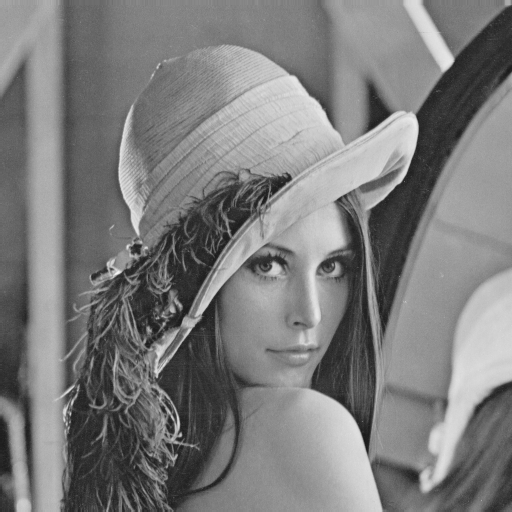
println("\n[1] Uploading an image...")
img_original = testimage("lena_gray_512")
img_original = Float64.(img_original)  
display(Gray.(img_original))

[1] Загрузка изображения...

┌ Warning: Usage of "lena" is not recommended, and the image may be removed in a later release. See https://womenlovetech.com/losing-lena-why-we-need-to-remove-one-image-and-end-techs-original-sin/ for more information.
└ @ TestImages /usr/local/ijulia-demos/packages/TestImages/UtVkc/src/TestImages.jl:124

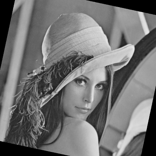
println("\n[2] Transformation (rotation + scale)...")
angle = π/15
scale = 1.0
center = SVector(size(img_original, 2)/2, size(img_original, 1)/2)
tfm = Translation(center) ∘ LinearMap(RotMatrix(angle)) ∘ LinearMap(SDiagonal(scale, scale)) ∘ Translation(-center)

img_transformed = warp(img_original, tfm, axes(img_original))
img_transformed = replace(img_transformed, NaN => 0.0, Inf => 0.0, -Inf => 0.0)
img_transformed_gray = Gray.(clamp01.(img_transformed))
display(img_transformed_gray)

[2] Трансформация (поворот + масштаб)...

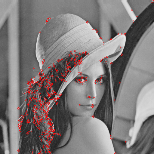
println("\n[3] Key point detection (Harris corners)...")
keypoints_original = harris_corners(img_original)
keypoints_transformed = harris_corners(img_transformed)
keypoints_transformed = filter_valid_keypoints(img_transformed, keypoints_transformed)

println("   Key points on the original: $(length(keypoints_original))")
println("   Key points on the transformed (valid): $(length(keypoints_transformed))")

img_kp_original = RGB.(img_original)
for (x,y) in keypoints_original
    draw_circle!(img_kp_original, (x, y), 3, RGB(1,0,0))
end
display(img_kp_original)

img_kp_transformed = RGB.(img_transformed)
for (x,y) in keypoints_transformed
    draw_circle!(img_kp_transformed, (x, y), 3, RGB(0,0,1))
end
display(img_kp_transformed)

[3] Детекция ключевых точек (Harris corners)...
   Ключевых точек на исходном: 421
   Ключевых точек на трансформированном (валидных): 297

println("\n[4] Extracting descriptors (patch-based)...")
desc_orig, valid_idx_orig = extract_patch_descriptors(img_original, keypoints_original)
desc_trans, valid_idx_trans = extract_patch_descriptors(img_transformed, keypoints_transformed)

println("   Valid descriptors in the original: $(length(valid_idx_orig))")
println("   Valid descriptors on the transformed: $(length(valid_idx_trans))")

[4] Извлечение дескрипторов (patch-based)...
   Валидных дескрипторов на исходном: 421
   Валидных дескрипторов на трансформированном: 227

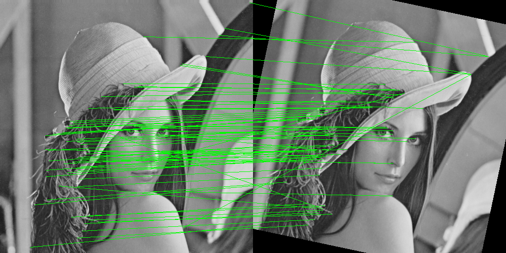
println("\n[5] Matching descriptors with ratio test...")
matches = match_descriptors_euclidean(desc_orig, desc_trans, valid_idx_orig, valid_idx_trans, ratio_thresh=0.7)
println("   Matches after ratio test: $(length(matches))")

h, w = size(img_original)
combined = fill(Gray(0), h, 2w)
combined[:, 1:w] = Gray.(img_original)
combined[:, w+1:2w] = img_transformed_gray
combined_rgb = RGB.(combined)

for (i1, i2) in matches
    x1, y1 = keypoints_original[i1]
    x2, y2 = keypoints_transformed[i2]
    p1 = (x1, y1)
    p2 = (x2 + w, y2)  
    draw_line!(combined_rgb, p1, p2, RGB(0,1,0))
end
display(combined_rgb)

[5] Сопоставление дескрипторов с ratio test...
   Совпадений после ratio test: 73

println("\n[6] RANSAC...")
inliers, H = ransac_homography(keypoints_original, keypoints_transformed, matches, iter=1000, thresh=3.0)
println("   Matches after RANSAC (inliers): $(length(inliers))")

combined_ransac = RGB.(combined)
for (i1, i2) in inliers
    x1, y1 = keypoints_original[i1]
    x2, y2 = keypoints_transformed[i2]
    p1 = (x1, y1)
    p2 = (x2 + w, y2)
    draw_line!(combined_ransac, p1, p2, RGB(0,1,0))
    draw_circle!(combined_ransac, p1, 5, RGB(1,0,0))
    draw_circle!(combined_ransac, p2, 5, RGB(1,0,0))
end
display(combined_ransac)

[6] RANSAC...
   Совпадений после RANSAC (inliers): 61

This article presents ** a complete computer vision training example** in the Julia language, which implements the classic pipeline for detecting and matching key points from scratch. Unlike using ready-made libraries (OpenCV, VLFeat), each algorithm is implemented manually with a detailed explanation of the mathematical basis.

Implemented components:

Component	Algorithm	Lines of Code
Rendering	Canvas (line, circle)	~60
Detection	Harris-Stevens	~40
Descriptors	Patch-based + Z-score	~35
Matching	Euclidean + Ratio Test	~20
Evaluation of the model	RANSAC + Homography	~50

Total: ~200 lines of code that demonstrate the full cycle from pixels to a geometric model.

Conclusion

This code demonstrates that understanding the fundamental algorithms of computer vision is more important than the ability to use ready-made libraries.
Use this code as a basis for your own experiments — change the parameters, try different images, add scale invariance, or integrate with ready-made descriptors. The understanding gained here will become the foundation for working with any computer vision systems.

Key point detection and matching

, Visualization of the detector operation

⚙️ Параметры и их влияние

Пошаговый разбор кода

Шаг 1: Подготовка изображения

Шаг 2: Вычисление градиентов (Оператор Собеля)

Step 3: Squares and products of gradients

Step 4: Smoothing with Window filter

Step 5: Calculating the Harris Response

Step 6: Threshold Filtering

Step 7: Non-Maximum Suppression

The final validity condition

Parameters and their impact

Step-by-step code analysis

Step 1: Getting the image dimensions

Step 2: Check the borders of the image

Step 3: Checking the pixel intensity

Step 4: Coordinate Conversion

Extracting descriptors based on patches: extract_patch_descriptors

The mathematical basis of descriptors

What is a descriptor?

Patch-based approach

Step 6: Normalization of the descriptor (Z-score)

Step 7: Assembling the Descriptor Matrix

Step 8: Processing the empty result

, Parameters and their impact

Step-by-step code analysis

Step 1: Image Preparation

Step 2: Calculating the offset for centering

Step 3: Coordinate Restriction (Clamping)

Step 4: Extract the patch

Step 5: Filtering low-quality patches

Сопоставление дескрипторов с Ratio Test: match_descriptors_euclidean

Математическая основа сопоставления

Задача сопоставления (Matching Problem)

Евклидово расстояние как метрика схожести

Ratio Test Лоу (1999)

, Parameters and their impact

Step-by-step code analysis

Step 1: Check for empty descriptors

Шаг 2: Перебор всех дескрипторов первого изображения

Шаг 3: Вычисление расстояний до всех кандидатов

Шаг 4: Поиск ближайшего соседа

Шаг 5: Сортировка расстояний для Ratio Test

Step 6: Applying the Ratio Test

Оценка гомографии через RANSAC: ransac_homography

Математическая основа

Что такое гомография?

Минимальное число точек

Линейная система для гомографии

The RANSAC algorithm

⚙️ Параметры и их влияние

Пошаговый разбор кода

Шаг 1: Проверка минимального числа совпадений

Шаг 2: Случайная выборка 4 точек

Шаг 3: Построение матрицы системы

Шаг 4: Решение системы уравнений

Шаг 5: Подсчёт inliers

Шаг 6: Обновление лучшей модели

Шаг 7: Возврат результата

Launch and visualization of all stages

, What this code demonstrates

Conclusion

Extracting descriptors based on patches: `extract_patch_descriptors`

Сопоставление дескрипторов с Ratio Test: `match_descriptors_euclidean`

Оценка гомографии через RANSAC: `ransac_homography`