Analysis of modulation schemes
This study presents a systematic approach to the implementation and verification of test models of receiving and transmitting paths in the Engee environment. The work includes a sequential analysis of various aspects of modulation schemes, starting with basic characteristics and ending with spectral properties.
Auxiliary model management function
To ensure correct operation with models, the function is implemented run_model, which automates the process of loading and executing models. The function performs the following operations:
-
Generates the full path to the model file with the extension
.engee -
Checks the current state of the model in the system core
-
Downloads a model from a file, if necessary, or opens an already uploaded one.
-
Runs the model and outputs detailed information about the process
-
Ensures that the work with the model is completed correctly
-
Returns execution results
This approach guarantees stable operation regardless of the initial state of the system.
function run_model( name_model)
    Path = (@__DIR__) * "/" * name_model * ".engee"
    if name_model in [m.name for m in engee.get_all_models()]
        model = engee.open( name_model )
        model_output = engee.run( model, verbose=true );
    else
        model = engee.load( Path, force=true )
        model_output = engee.run( model, verbose=true );
        engee.close( name_model, force=true );
    end
    sleep(0.1)
    return model_output
end
Bit error probability analysis
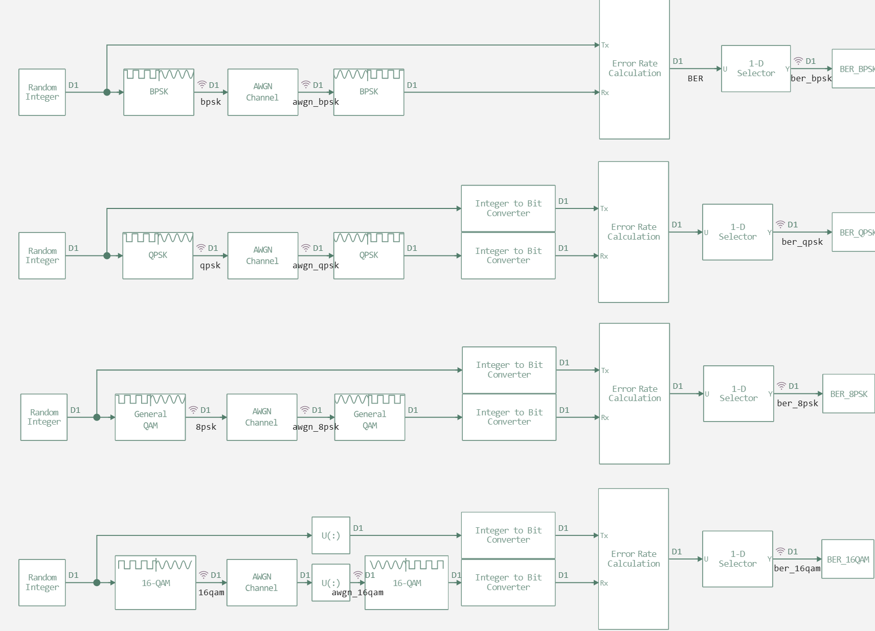
A comparative study of the characteristics of four modulation schemes was carried out: BPSK, QPSK, 8-PSK and 16-QAM. The research methodology includes:
-
Simulation in the signal-to-noise ratio (Eb/No) range from 0 to 10 dB in 2 dB increments
-
Theoretical calculation of BER characteristics using mathematical models for each modulation
-
Visualization of results on a logarithmic scale for visual comparison
A basic model containing identical signal processing paths for all modulations was used, which ensures the correctness of the comparative analysis, the model itself is demonstrated below.
EbNoArr = collect(0:2:10);
Eb_No = 0;
ber_bpsk = zeros(length(EbNoArr));
ber_8psk = zeros(length(EbNoArr));
ber_qpsk = zeros(length(EbNoArr));
ber_16qam = zeros(length(EbNoArr));

for i in 1:length(EbNoArr)
    Eb_No = EbNoArr[i]

    run_model("modulations_1");

    ber_bpsk[i] = collect(BER_BPSK).value[end][1]
    ber_8psk[i] = collect(BER_8PSK).value[end][1]
    ber_qpsk[i] = collect(BER_QPSK).value[end][1]
    ber_16qam[i] = collect(BER_16QAM).value[end][1]
end
using SpecialFunctions
colors = Dict(:BPSK => :blue, :QPSK => :red, :PSK8 => :green, :QAM16 => :purple)
function theoretical_ber(EbNo_dB, mod_type)
    EbNo = 10 .^ (EbNo_dB ./ 10)
    if mod_type == :BPSK
        0.5 .* erfc.(sqrt.(EbNo))
    elseif mod_type == :QPSK
        0.5 .* erfc.(sqrt.(EbNo))
    elseif mod_type == :PSK8
        (2/3) .* erfc.(sqrt.(3*EbNo) .* sin(π/8))
    elseif mod_type == :QAM16
        (3/8) .* erfc.(sqrt.(2 .* EbNo ./ 5))
    end
end
EbNoArr_dense = range(minimum(EbNoArr), maximum(EbNoArr), length=1000)
plot(yscale=:log10, ylims=(1e-6, 1), grid=true, xlabel="Eb/No (dB)", ylabel="BER", title="Theoretical and simulated BER")

for mod in [(:BPSK, ber_bpsk), (:QPSK, ber_qpsk), (:PSK8, ber_8psk), (:QAM16, ber_16qam)]
    mod_type, ber_sim = mod
    c = colors[mod_type]
    plot!(EbNoArr_dense, theoretical_ber(EbNoArr_dense, mod_type), line=:solid, color=c, label="$mod_type (theory)")
    scatter!(EbNoArr, ber_sim, marker=:circle, color=c, label="$mod_type (simul.)", markersize=5)
end
plot!(legend=:bottom)
Analysis of power characteristics and signal constellations
The study was expanded by using a model with Nyquist filters in the receiving and transmitting paths. The analysis was carried out:
-
Signal strengths before and after filtering to assess the effect of filters
-
Signal constellations demodulated signals for visual assessment of demodulation quality
Constellations for all considered modulation schemes with reference points are constructed.
\ The model itself is presented below.
.png)
run_model("modulations_2")
using Statistics
println("Before the filter:")
bpsk = collect(simout["modulations_2/bpsk"]).value
power_bpsk = mean(abs2.(x[1]) for x in bpsk)
println("BPSK Power: $power_bpsk")

qpsk = collect(simout["modulations_2/qpsk"]).value
power_qpsk = mean(abs2.(x[1]) for x in qpsk)
println("QPSK Power: $power_qpsk")

psk8 = collect(simout["modulations_2/8psk"]).value
power_8psk = mean(abs2.(x[1]) for x in psk8)
println("8PSK Power: $power_8psk")

qam16 = collect(simout["modulations_2/16qam"]).value
power_16qam = mean(abs2.(x[1]) for x in qam16)
println("16QAM Power: $power_16qam")

println("After the filter:")
bpsk = collect(simout["modulations_2/bpsk_f"]).value
power_bpsk = mean(abs2.(x[1]) for x in bpsk)
println("BPSK Power: $power_bpsk")

qpsk = collect(simout["modulations_2/qpsk_f"]).value
power_qpsk = mean(abs2.(x[1]) for x in qpsk)
println("QPSK Power: $power_qpsk")

psk8 = collect(simout["modulations_2/8psk_f"]).value
power_8psk = mean(abs2.(x[1]) for x in psk8)
println("8PSK Power: $power_8psk")

qam16 = collect(simout["modulations_2/16qam_f"]).value
power_16qam = mean(abs2.(x[1]) for x in qam16)
println("16QAM Power: $power_16qam")
Let's perform the construction of a guide for each of the modulations.
bpsk = collect(simout["modulations_2/bpsk_demod"]).value
bpsk = [x[1] for x in bpsk]  # Extracting the first element of each vector
plot(title="BPSK")
plot!(bpsk, seriestype=:scatter)
plot!([-1+0im, 1+0im], seriestype=:scatter)
qpsk = collect(simout["modulations_2/qpsk_demod"]).value;
qpsk = [x[1] for x in qpsk]  # Extracting the first element of each vector
plot(title="QPSK")
plot!(ComplexF64.(qpsk), seriestype=:scatter)
plot!([0.75+0.75im, 0.75-0.75im, -0.75+0.75im, -0.75-0.75im], seriestype=:scatter)
psk8 = collect(simout["modulations_2/8psk_demod"]).value;
psk8 = [x[1] for x in psk8]  # Extracting the first element of each vector
plot(title="8-PSK")
plot!(ComplexF64.(psk8), seriestype=:scatter)
plot!(cis.(2pi*[0:7...]/8), seriestype=:scatter)
qam16 = collect(simout["modulations_2/16qam_demod"]).value;
qam16 = [(i...)+0 for i in qam16];
plot(title="16QAM")
plot!(ComplexF64.(qam16), seriestype=:scatter)
plot!([a + b*im for a in -3:2:3, b in -3:2:3][:], seriestype=:scatter)
Spectral analysis of modulated signals
For an in-depth study of the properties of modulated signals, we performed:
-
Calculation of the spectral power density using:
-
Hanning window function to reduce spectral leakage effects
-
Median filtering for smoothing spectral characteristics
-
-
Comparison with the theoretical model of the Nyquist spectrum with a smoothing coefficient of 0.2
-
Visualization of spectral characteristics in the frequency domain
The implemented model demonstrates the possibilities of analyzing multi-frequency systems using data buffering.
.png)
using FFTW, DSP, Statistics, SpecialFunctions

function compute_smoothed_spectrum(signal, fs, window_size=20)
    window = hanning(length(signal))
    windowed_signal = signal .* window
    power_spectrum = abs.(fft(windowed_signal)).^2 / (sum(abs2, window) * fs)
    power_spectrum_db = 10*log10.(power_spectrum)

    function my_medfilt(signal, window_size)
        half_window = window_size ÷ 2
        smoothed = similar(signal)
        n = length(signal)
        for i in 1:n
            start_idx = max(1, i - half_window)
            end_idx = min(n, i + half_window)
            window_data = signal[start_idx:end_idx]
            smoothed[i] = median(window_data)
        end
        return smoothed
    end
    power_spectrum_db_smoothed = my_medfilt(power_spectrum_db, window_size)
    freqs = fftfreq(length(signal), fs)
    return fftshift(freqs), fftshift(power_spectrum_db_smoothed)
end

function nyquist_spectrum(frequencies, rolloff_factor=0.5, symbol_rate=1.0)
    T = 1.0 / symbol_rate
    f_N = 1.0 / (2 * T)
    spectrum = zeros(length(frequencies))
    for (i, f) in enumerate(frequencies)
        f_abs = abs(f)
        if f_abs <= (1 - rolloff_factor) * f_N
            spectrum[i] = T
        elseif f_abs <= (1 + rolloff_factor) * f_N && f_abs > (1 - rolloff_factor) * f_N
            spectrum[i] = T/2 * (1 + cos(π * T / rolloff_factor * (f_abs - (1 - rolloff_factor) * f_N)))
        else
            spectrum[i] = 0.0
        end
    end
    spectrum_db = 10 * log10.(spectrum .+ 1e-12)
    return spectrum_db
end

fs = 400
window_size = 15
symbol_rate = 50.0
rolloff = 0.2

run_model("modulations_3")

bpsk = collect(simout["modulations_3/bpsk_f"]).value
bpsk = [(i...)+0 for i in bpsk]
qpsk = collect(simout["modulations_3/qpsk_f"]).value
qpsk = [(i...)+0 for i in qpsk]
psk8 = collect(simout["modulations_3/8psk_f"]).value
psk8 = [(i...)+0 for i in psk8]
qam16 = collect(simout["modulations_3/16qam_f"]).value
qam16 = [(i...)+0 for i in qam16]

freqs_bpsk, spectrum_bpsk = compute_smoothed_spectrum(bpsk, fs, window_size)
freqs_qpsk, spectrum_qpsk = compute_smoothed_spectrum(qpsk, fs, window_size)
freqs_psk8, spectrum_psk8 = compute_smoothed_spectrum(psk8, fs, window_size)
freqs_qam16, spectrum_qam16 = compute_smoothed_spectrum(qam16, fs, window_size)
freqs_theoretical = range(-fs/2, fs/2, length=1000)
spectrum_nyquist_02 = nyquist_spectrum(freqs_theoretical, 0.2, symbol_rate)
max_experimental = maximum([maximum(spectrum_bpsk), maximum(spectrum_qpsk), maximum(spectrum_psk8), maximum(spectrum_qam16)])
max_theoretical_02 = maximum(spectrum_nyquist_02)
spectrum_nyquist_02_normalized = spectrum_nyquist_02 .- (max_theoretical_02 - max_experimental)

plot(freqs_bpsk, spectrum_bpsk, label="BPSK", linewidth=2, grid=true)
plot!(freqs_qpsk, spectrum_qpsk, label="QPSK", linewidth=2)
plot!(freqs_psk8, spectrum_psk8, label="8-PSK", linewidth=2)
plot!(freqs_qam16, spectrum_qam16, label="16-QAM", linewidth=2)
plot!(freqs_theoretical, spectrum_nyquist_02_normalized, label="Nyquist α=0.2", linewidth=3, linestyle=:dash, color=:red)
title!("Energy spectrum of modulated signals (fs = $fs Hz)\nmedian filter with window $window_size")
xlabel!("Frequency, Hz")
ylabel!("Spectral power density, dB/Hz")
xlims!(-fs/2, fs/2)
The results obtained make it possible to conduct a comprehensive analysis of the modulation schemes and justify the choice of optimal modulation for specific operating conditions of communication systems.
Conclusion.
Based
on a comprehensive analysis of the characteristics of the modulation schemes, the following conclusions can be drawn.
| Parameter | BPSK | QPSK | 8-PSK | 16-QAM |
|---|---|---|---|---|
| Effectiveness | 1 b/s/Hz | 2 b/s/Hz | 3 b/s/Hz | 4 b/s/Hz |
| Required Eb/No for BER=10-3 | ~7 dB | ~7 dB | ~11 dB | ~15 dB |
| The complexity of demodulation | Low | Low | Average | High |
Best choice for different scenarios:
- For maximum noise immunity → BPSK
- Optimal compromise → QPSK ⭐
- With limited bandwidth and good SNR → 8-PSK
- For maximum speed in ideal conditions → 16-QAM
To summarize, QPSK is the most balanced and practical choice for most real-world communication systems, providing the optimal ratio of noise immunity, spectral efficiency, and ease of implementation. BPSK should be used in systems with extreme reliability requirements, and higher-level modulations should only be used with guaranteed good communication channel quality.