Image classification using a convolutional neural network

In this project, we are training a convolutional neural network to classify images of several classes. At the output, we get a trained algorithm that takes an image as input and returns a prediction of the class to which it may belong.

Let's prepare the environment

We will install the necessary packages and configure the environment to display static graphs. In case of problems with libraries, run the command EngeePkg.purge(), which will eliminate all packages except system packages from your system and will allow you to install the necessary packages without compatibility problems.

# Installing the necessary packages
Pkg.add(["Flux", "BSON", "ImageTransformations"])
gr();

The training data is located in several folders in the "training data" directory. Folder names are read from the file system and become class names. We also indicate where the examples for classification (with unknown labels) are located.

DATA_DIR = "$(@__DIR__)/training data";
UNKNOWN_DIR = "$(@__DIR__)/unknown";

Model training and validation

In this project, we will train a convolutional model of the following type from scratch:

In the script train.jl The functions that carry out are collected:

Uploading images from class folders, resizing to 128x128, normalization
Calculating the imbalance of classes (how many forks, how many spoons)
Division of data into train/test (stratified, 75%/25%)
** Model Assembly** — convolutional network with BatchNorm and Dropout
Balanced batches — so that in each butch had both classes equally
Augmentation — doubling samples in the dataset by reflection and highlighting
Learning cycle — forward pass, loss calculation, backward pass, weight update
Quality assessment — accuracy, precision, recall on the test
Early stopping — stop if there are no improvements 8 epochs
Saving the best model

include("$(@__DIR__)/_scripts/train.jl")
model, classes = train_model(DATA_DIR; epochs=25, batch_size=16, lr=0.0005, test_split=0.25);

Batch size: 16, Learning rate: 0.0005
Percentage of the test sample: 25.0%
Найдено классов: 2: ["fork", "spoon"]

=== Class distribution ===

Total images: 335 (128×128)
  Fork: 189 images (56.4%)
  spoon: 146 images (43.6%)

=== Data separation ===
  Training: 252 (75.2%)
  Test results: 83 (24.8%)
Model parameters: 607810

=== Training ===
  Epoch 1/25, Train Loss: 1.3937, Train Acc: 44.4%, Test Acc: 44.6% ★ (precision/recall by class: fork: 65.2%/31.9%, Spoon: 46.7%/77.8%)
  Epoch 2/25, Train Loss: 1.3289, Train Acc: 48.0%, Test Acc: 42.2% (precision/recall by class: fork: 75.0%/12.8%, spoon: 45.3%/94.4%)
  Epoch 3/25, Train Loss: 1.3427, Train Acc: 66.3%, Test Acc: 61.4% ★ (precision/recall by class: fork: 63.8%/78.7%, Spoon: 60.0%/41.7%)
  Epoch 4/25, Train Loss: 1.1816, Train Acc: 57.1%, Test Acc: 49.4% (precision/recall by class: fork: 72.7%/17.0%, spoon: 45.8%/91.7%)
  Epoch 5/25, Train Loss: 1.1303, Train Acc: 79.0%, Test Acc: 75.9% ★ (precision/recall by class: fork: 71.7%/80.9%, spoon: 70.0%/58.3%)
  Epoch 6/25, Train Loss: 1.0433, Train Acc: 73.4%, Test Acc: 68.7% (precision/recall by class: fork: 77.8%/74.5%, spoon: 68.4%/72.2%)
  Epoch 7/25, Train Loss: 0.9447, Train Acc: 78.2%, Test Acc: 67.5% (precision/recall by class: fork: 78.0%/68.1%, spoon: 64.3%/75.0%)
  Epoch 8/25, Train Loss: 0.9592, Train Acc: 79.4%, Test Acc: 73.5% (precision/recall by class: fork: 90.6%/61.7%, spoon: 64.7%/91.7%)
  Epoch 9/25, Train Loss: 1.0558, Train Acc: 84.1%, Test Acc: 75.9% (precision/recall by class: fork: 93.8%/63.8%, Spoon: 66.7%/94.4%)
  Epoch 10/25, Train Loss: 0.8999, Train Acc: 81.3%, Test Acc: 67.5% (precision/recall by class: fork: 78.9%/63.8%, spoon: 62.2%/77.8%)
  Epoch 11/25, Train Loss: 0.97, Train Acc: 86.5%, Test Acc: 75.9% (precision/recall by class: fork: 78.3%/76.6%, spoon: 70.3%/72.2%)
  Epoch 12/25, Train Loss: 0.8364, Train Acc: 89.3%, Test Acc: 75.9% (precision/recall by class: fork: 82.9%/72.3%, spoon: 69.0%/80.6%)
  Epoch 13/25, Train Loss: 0.7675, Train Acc: 79.4%, Test Acc: 66.3% (precision/recall by class: fork: 67.7%/89.4%, spoon: 76.2%/44.4%)

   Early shutdown after 13 epochs (no improvement for 8 epochs)

The best model loaded (Test Acc: 75.9%)

=== Results ===
  Better accuracy on the test: 75.9%

  Train/test accuracy: 78.2% / 72.3%
  ✓ No retraining (5.9% gap)
The training is completed! 🚀
The model is saved in model.bson

After training, we will transform how the model behaves. The script performs the following steps:

Loading the model, metadata, and unknown images — The network architecture, weights, class names, and number of examples in each class of the training set are extracted from the BSON file, and the model is switched to evaluation mode. The specified folder is scanned, each image is reduced to a size of 128×128, normalized to the range [-1, 1] and converted to the tensor format W×H×C
Classification of each image — the tensor is fed to the input of the model, the output logits are converted into probabilities via softmax, the class with the maximum probability and the corresponding confidence are determined, and the grouping by classes
Sorting by confidence and statistics output — Within each class, images are sorted from the most confident predictions to the least confident. Number of predicted images, percentage of total, average, maximum and minimum confidence
Bias analysis — comparison of the percentage of predictions of each class with the percentage of this class in the training set, indicator output

include("$(@__DIR__)/_scripts/visualize.jl")
results = classify_and_visualize(UNKNOWN_DIR);

=== Statistics of the training set ===
  Fork: 189 images
  spoon: 146 images

=== Classification results ===
  fork:
    Quantity: 5 (50.0%)
    Average confidence: 0.902
    Max/min confidence: 1.0 / 0.752
  spoon:
    Quantity: 5 (50.0%)
    Average confidence: 0.626
    Max/min confidence: 0.692 / 0.578

=== Bias analysis ===
  fork: 50.0% predicted vs 56.4% trained ✓
  spoon: 50.0% predicted vs 43.6% trained ✓

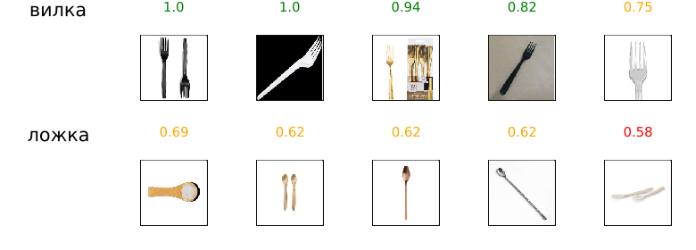
We will classify all the images from the "unknown" folder and output up to 10 images for each class.

include("$(@__DIR__)/_scripts/simple_mosaic.jl")
plot(create_simple_mosaic(UNKNOWN_DIR))

The following script allows you to reopen the trained model, predict the class for all files from the catalog of unlabeled examples, and output the results to a table.

include("$(@__DIR__)/_scripts/predict_to_csv.jl")
predict_to_csv(UNKNOWN_DIR, confidence_threshold=0.6, output_csv="$(@__DIR__)/predictions.csv")

Processed files: 10
  Fork: 5
  Spoon: 4
  Unknown: 1

Saved in /user/_retrain_resnet/predictions.csv

Conclusion

The project has built the foundation for a simple task: arrange images in several folders and train a classifier that will allow you to distribute images from a second folder with unknown objects into the same classes.

The results presented in the example are obtained using a neural network that has gone through dozens of iterations of the learning process. To get a good classification algorithm, you need to vary hyperparameters, study the dataset, change the duration of training, the topology of the neural network (more layers, turn on or off batch normalization, etc.), the size of the batches or the optimizer, remove the barrier of premature shutdown, or simply change the settings of the random number generator.

Row	Файл	Предсказанный_класс	Уверенность	Вероятность_вилка	Вероятность_ложка
	String	String	Float32	Float32	Float32
1	00000495.jpg	вилка	0.999757	0.999757	0.000242674
2	00000496.png	вилка	0.995816	0.995816	0.00418395
3	00000494.jpg	вилка	0.936342	0.936342	0.0636576
4	00000497.jpg	вилка	0.824374	0.824374	0.175625
5	00000498.jpg	вилка	0.752225	0.752225	0.247775
6	00000194.jpg	ложка	0.692343	0.307657	0.692343
7	00000193.png	ложка	0.62094	0.37906	0.62094
8	00000196.jpg	ложка	0.618481	0.381519	0.618481
9	00000195.jpg	ложка	0.618284	0.381716	0.618284
10	00000192.jpg	неизвестно	0.577928	0.422072	0.577928