Optimization of flow distribution in queuing systems
In today's digital world, from global data networks to logistics chains and transaction processing systems, we are constantly faced with the need for effective flow management. How to ensure uninterrupted operation of Internet connections during peak loads? How to optimize the routes of delivery of goods in a megalopolis? How can I design a call center so that customers don't have to wait for a response? The answers to these questions lie in the field of queuing theory, a mathematical discipline that studies systems where requests (data packets, customers, vehicles) arrive for service, forming queues.
Queuing Service System (QMS) it is a mathematical model consisting of service devices (channels, servers, nodes) and the flow of applications that these devices process. Of particular interest is the M/M/1 system, a fundamental model where the incoming flow of requests has a Poisson character (random, independent events with a constant average intensity), and the service time is subject to an exponential distribution (characterized by the "lack of memory" property). This simple but deep model reveals the paradoxical nature of queues: as the load approaches 100%, the queue length increases hyperbolically rather than linearly, making optimization not just desirable, but critically necessary.
Network CFOs are the next level of complexity, where many service nodes are connected to a network. Such a system is naturally described by a directed graph, where nodes represent processing points, and branches represent communication channels with limited bandwidth. For the mathematical representation of the network structure, the adjacency matrix (describing the presence of connections between nodes) and the incidence matrix (fixing the directions of these connections) are used. It is these mathematical objects that become the building blocks for setting the optimization problem.
But how to find the optimal distribution of flows in a complex network? How can information flows or vehicles be directed in such a way as to minimize the average waiting time in the system, while avoiding overloading individual channels? This problem is solved using nonlinear optimization, where the objective function is the sum of the average numbers of requests in all channels (derived from the formula for M/M/1), and constraints include the balance of flows in nodes and physical limitations of throughput.
In this paper, we present a complete cycle of network CFM analysis and optimization, from theoretical foundations to practical implementation in the Engee environment. You will see how:
-
Convert real data about throughput and flows into mathematical models;
-
Visualize complex network structures using graphs;
-
Formulate an optimization problem with hundreds of variables and constraints;
-
Solve it using modern nonlinear optimization algorithms;
-
Analyze the results through interactive visualizations and quantitative metrics.
In this example, we do not limit ourselves to theoretical calculations, but go through the entire process — from the source data in Excel format to ready-made recommendations for network optimization, accompanying each step with visual graphs and detailed explanations. Using Julia, a language that combines the speed of C with the expressiveness of Python, makes the solution both efficient and transparent.
We will attach the necessary libraries.
using XLSX, JuMP, Ipopt, DataFrames, Graphs, SimpleWeightedGraphs, Colors, Printf, LinearAlgebra, Printf, GraphPlot
We will attach the necessary function files.
foreach(include, ("opti1.jl", "opti2.jl", "opti3.jl", "opti4.jl", "opti5.jl", "opti6.jl", "opti7.jl", "opti8.jl", "opti9.jl", "flowDir.jl", "optiwrite.jl", "lfwrite.jl"))
foreach(include, ("readqs.jl", "flowGraph.jl", "flGplot.jl", "netGraph.jl", "simpGraph.jl", "sGplot.jl","nGplot.jl"))
CFR structure
The structure of the queuing system can be represented as a square network matrix with a diagonal size of zero :
Where – the number of nodes in the network, – the total bandwidth of communication channels (graph branches) connecting nodes and directed from the node with the number to the node with the number , and the zero diagonal implies the absence of channels for information flows from the node addressed to itself.
The flow direction in queuing systems can also be represented as a square matrix with a diagonal of zero in size. :
Where – the number of nodes in the network, – the amount of flow directed from the node with the number to the node with the number . The zero diagonal in the matrix implies the absence of flows from the node addressed to itself.
Flows and throughput capacities can be represented by any unit of measurement used in queuing systems, for example: Mbit/s, the number of products per hour; the number of goods transported per day; the number of vehicles driven per hour, the number of requests per day, etc..
Initial data
In our example, the source data is presented in the form of xlsx tables. NetMatrix.xlsx — bandwidth and direction of communication lines, FlowMatrix.xlsx — the intensity and direction of the flows.
Let's read the source data.
СМО = readqs("NetMatrix.xlsx", 1);
Потоки = readqs("FlowMatrix.xlsx", 1);
Let's display the capacities of the communication lines as a matrix.
display(CFR)
Let's display the flows as a matrix.
display(Streams)
Based on the initial data, we will determine the number of nodes, streams, and communication lines in the CFR under study.
nodes = size(CFR, 1);
lines = count(!iszero, CFR);
threads = count(!iszero, Threads);
println("In a queuing system\n\nodes: $nodes\nstreams: $streams\lines of communication: $lines")
Visualization of CFR
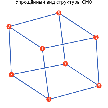
Let's display the CFR structure as a graph. For clarity, we will not take into account the directions and intensities of communication lines in this graph.
and, n = simpGraph(CFR);
Graph = sGplot(i, n)
display(Graph)
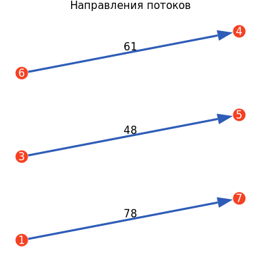
By specifying the node numbers, intensity values, and arrows, we will display the flow directions.
nfl, nl, flG, flI = flowGraph(Streams);
ГрафПотоков = flGplot(flG, flI, nl, "Flow directions");
display(Graph streams)
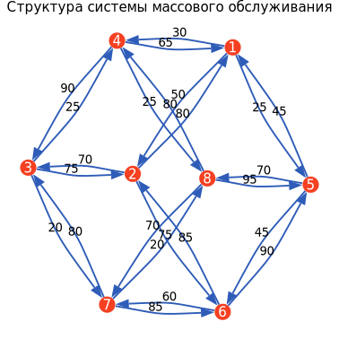
Now we will display the complete structure of the CFR in the form of a directed graph with node numbers, directions and capacities of communication lines.
s, t, bW = netGraph(CFR);
ГрафСМО = nGplot(s, t, bW, "The structure of the queuing system");
display(GRAPHSMO)
The M/M/1 system
Consider the M/M/1 system, in which the incoming flow of applications has a Poisson distribution, and the distribution of service time is exponential, then the average number of applications in the system is determined by the formula:
Where – the intensity of applications received, – bandwidth of communication lines. This formula arises due to randomness in the moments of arrival and service of applications. When the system is running close to its capacity limit (the load is approaching 100%), even small random delays begin to accumulate, causing hyperbolic, rather than linear, queue growth. Mathematically, this is a consequence of the geometric distribution of the number of applications in the system, the average value for which is determined by this expression. In the future, based on this formula, an objective function for optimization will be formed.
Transformation of the source data
For further solutions, we transform the bandwidth matrix into 3 vectors.:
- list of sources;
- List of receivers;
- a list of throughput capacities.
source, receiver, capacity = opti1(CFR, nodes, lines);
During the optimization process to bypass the loaded communication lines, the streams can be divided into fractions. The structure of the flow fractions can be represented as a system of matrices in the number of size :
Where – number of nodes, – number of streams, – the value of the flow fraction number passing through a line directed from node number to node number .
The incidence matrix
Based on the adjacency matrix, we will create an incidence matrix.
Each column corresponds to a branch of the graph: the source line contains -1, in the receiver line — +1. The matrix has the size узлов × линий and describes which nodes are connected by each edge and the direction of the lines.
Occurrence matrix = opti2(nodes, lines, source, receiver);
display(Occurrence matrix)
Flow restrictions
Let's transform the flow matrix into 3 vectors:
-
list of senders;
-
List of recipients;
-
List of flow intensities.
source, inflow, intensity = opti3(Flows, nodes, flows);
Let's create a matrix indicating the intensities of outgoing flows from source nodes and incoming flows to receiver nodes. The number of rows is equal to the number of nodes, and the number of columns is equal to the number of threads. A negative value indicates an outgoing flow from the source node, a positive value indicates an incoming flow to the receiver node. The row numbers correspond to the node numbers.
source_flow = opti4(nodes, flows, source, inflow, intensity);
display(source of supply)
Let's create a three-dimensional array indicating the flow directions in each communication line. The number of rows is two (source and inflow), the number of columns corresponds to the number of communication lines линий, and the number of two-dimensional matrices corresponds to the number of streams потоков. This array will be used to block incoming flows to source nodes and outgoing flows from receiver nodes.
Constraints = opti5(lines, streams, source, receiver, source, inflow);
display(restrictions)
Equations and inequalities
Based on the incidence matrix and the flow direction array, we will create a three-dimensional array indicating the signs (-1 or 0 or +1) of the flow fractions for the CFR optimization constraint equations. The number of lines corresponds to the number of nodes plus two, since an amount equal to the number of nodes indicates restrictions in the intermediate communication lines, and the last two in the terminal ones, which block incoming flows to the source nodes and outgoing from the receiver nodes. These arrays will be used to create optimization constraint equations.
Equations = opti6(nodes, occurrence matrix, lines, flows, constraints, source of inflows);
display(Equations)
By multiplying the resulting array element-wise by variables indicating the fractions of flows, we obtain a system of equations.
Let's consider how the equation is formed for node 1, flow . Representing the fractions of streams as a matrix:
Let's take an element of the matrix with the index which is equal to zero. The elements of the first row are substituted into the equation with a minus sign, the elements of the first column are substituted into the equation with a plus sign. We get the equation:
For the following nodes, take the indexes , and repeat the composition of the equations. These equations introduce constraints that mean that the sum of incoming and outgoing flows at intermediate nodes is zero.
For clarity, we will draw up a system of optimization constraint equations in a general way using the example of nodes.: and the flow :
Where – number of nodes, – the number of threads.
In addition to the systems of equations, the necessary limitation is the maximum intensity of the fraction of flows in the communication lines, which should not exceed their bandwidth. For a CFR consisting of 8 nodes and 24 communication lines, this constraint will be represented by the following system of inequalities:
We transform the obtained results into the initial data for performing the optimization task.
A, B, λ0, a, b = opti7(nodes, flows, lines, Equations, source_flow, capacity);
display(A)
display(B)
Target function
Based on the structure of the bandwidth matrix and the flow matrix, we will create an objective function. For a CFR consisting of 8 nodes, 24 communication lines and 3 streams, the objective function will have the following form:
The objective function can be represented in a general way:
where – the value of the average number of requests in the queuing system, – number of communication lines – number of streams, – the amount of bandwidth of the communication line directed from the node to the node , – the desired optimal intensity of the fraction of the flow directed from the node to the node , which is part of the stream .
The optimization task boils down to the following goal: to find such values , under which it will take the minimum value.
Optimization
Let's form the target function and complete the optimization task.
T, λ, load = opti8(A, B, λ0, a, b, capacity, flows);
Optimization results
We transform the data for display as graphs and output as xlsx tables. And in case of successful optimization, we will output the matrices of optimal flow distributions.
Optimal, load systems = opti9(streams, lines, λ, nodes, source, receiver, capacity);
if T # load > 0
display(Optimal)
end
Let's output the optimization results.
nl = flowDir(Streams);
if T
    optiwrite(Optimal, streams)
    println("\Optimization has been completed.\n")
    println("\Average number of requests in the system: $load\n")
else
    println("Optimization is not feasible with the given flow rates and capacities of communication lines.")
end
Let's create an xlsx file and output a matrix with the load coefficients of the communication lines.
lfwrite(Load systems)
display(Load systems)
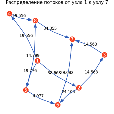
Visualization of optimal flows
If the optimization is performed, we will display the optimal distribution of flow intensities in the form of graphs.
if T
    fnums = reshape(nl, (2, threads));
    for m in 1:streams
    optiname = "Distribution of flows from node $(fnums[1, m]) to node $(fnums[2, m])"
    и, п, ё = netGraph(readqs("OptiFlows.xlsx", m));
    Optgraph(m) = nGplot(i, n, e, optiname);
    display(Optograph(m))
    end
else
    println("It is necessary to increase the capacity of communication lines or reduce the intensity of flows.\n")
end
.png)
.png)
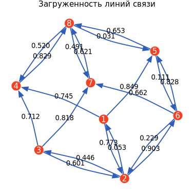
Visualization of line congestion
Let's display the load coefficients of the communication lines in the form of a graph. Based on this graph, it is possible to analyze whether certain communication lines require an increase in bandwidth. If optimization is not feasible with a given bandwidth of communication lines, load factors exceeding one indicate how many times this communication line needs to be increased in order for optimization to become possible.
lM = readqs("LoadFactors.xlsx", 1);
s1, t1, bW1 = netGraph(lM);
ГрафНагрузки = nGplot(s1, t1, bW1, "Congestion of communication lines");
display(Loading graph)
In addition to the graphs presented, we obtained xlsx tables with optimal flow distribution matrices as calculation results (OptiFlows.xlsx ) and the load of communication lines at these values of flows and capacities of communication lines (LoadFactors), which will be convenient to use for further calculations and research.
Optimize your own system
With the help of the presented algorithm, you can optimize your own queuing system, for this:
-
Prepare two standardized Excel files.:
-
NetMatrix.xlsx— matrix of directions and transmission capacities of communication lines -
FlowMatrix.xlsx— a matrix of the directions and intensities of the serviced flows
-
-
Upload them to an interactive computing environment
-
Initiate an analytical process to obtain a comprehensive result.:
-
Optimal distribution matrices for each flow
-
Graphical representation of channel loading coefficients
-
Visualization of network topology and flow configuration
-
Quantitative indicators of system parameters
-
Regardless of the scale and specifics of the system, whether it is a municipal transport infrastructure, a corporate computer network, or a production and logistics complex, the presented tool provides adaptive analysis based on the data provided. The methodology makes it possible to identify critical elements operating at the capacity limit, identify underloaded routes, and determine optimal flow distribution schemes.
It should be noted that optimization of network structures is no longer the exclusive competence of specialists with access to specialized software. Currently, this is becoming a standardized procedure in which complex computational algorithms are implemented in an intuitive interface, and the depth of analytics is organically combined with the visual presentation.
It is recommended to test the methodology on current data. Uploading the matrices of a specific system to the Engee environment will allow you to observe the practical implementation of the principles of queuing theory, discover hidden reserves in existing configurations, and find effective solutions for optimization problems.
Optimization should be considered not as a one-time event, but as a continuous improvement process. The presented toolkit ensures its consistency, visibility and effectiveness, forming the basis for making informed management decisions in a dynamic environment of complex network systems.
Conclusion
The present study has demonstrated a methodological transition from the fundamental principles of queuing theory to the practical implementation of integrated optimization of network structures. Using the example of a system comprising 8 nodes, 24 communication channels and 3 service streams, the transformation of mathematical concepts — Poisson flows, exponential distributions, adjacency and incidence matrices — into effective tools for solving applied problems was illustrated. The M/M/1 model, which is a classic object of theoretical consideration, has been successfully applied as a basis for constructing an objective function that minimizes the average number of requests in a distributed network.
The central result of the work carried out is to demonstrate that optimization of network structures is a systematic process with well-defined stages: mathematical modeling, visual representation, constraint formalization, numerical solution and analytical interpretation of the results. It has been experimentally confirmed that even in networks of moderate complexity, information flows are naturally distributed along alternative routes, demonstrating adaptability to potential overloads of critical elements. Visualization of the results through directed graphs provided not only a representation of the final values, but also an understanding of the cause-and-effect relationships in the system.
The most significant aspect is the practical accessibility of the presented methodology. A ready-made instrumental solution is offered for specialists who solve the problems of designing telecommunication networks, optimizing logistics routes, allocating computing resources or managing information flows.