Optimization of pipeline geometry
In this project, we optimize the parameters of the pipeline geometry to achieve the desired flow parameters.
Let's consider a simple model where a T-shaped branching occurs in a pipeline, followed by two curved pipes. By changing their bending angle in the range from 0 to 120 degrees, we will achieve a given cost difference through each branch of the system.
Description of the model
Download several libraries:
Pkg.add("Optim")
using DataFrames, CSV, Optim
Let's open our model.
engee.open( "$(@__DIR__)/" * "pipe_circuit_optimization.engee");
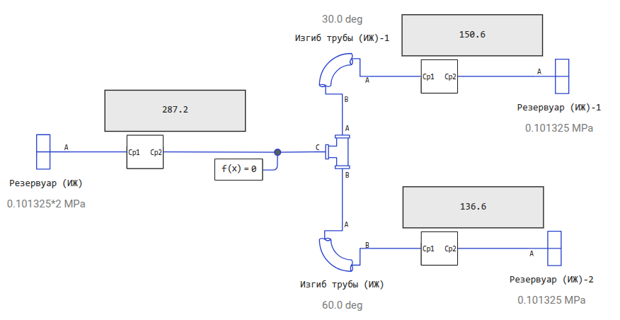
When the bending of both pipes is the same, the same flow rate of liquid flows through each pipe, equal to half of the inlet flow.
Optimization of model parameters
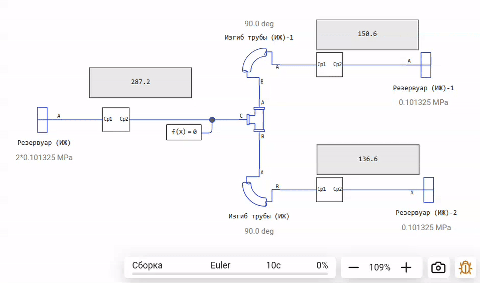
Let's formulate the problem in a fairly simple way: we pre-launched a model in which the bending of the pipes was equal to 30 and 60 degrees. We will set the obtained values as target optimization criteria (consumption 150.6 and 136.6 kg/s) and set the initial bending values of each pipe to 90 degrees.
The optimization task will require the definition of free variables ("independent" ones, whose values we will gradually change) and dependent variables (with target values).
Free variables are some internal properties of some blocks with target values and physical constraints.
cd( @__DIR__ )
adj = CSV.read("adjustable_parameters.csv", DataFrame)
Dependent variables are the desired values of some signals at the final moment in time.
tgt = CSV.read("target_parameters.csv", DataFrame)
Let's start the optimization process, during which we will look for the values of the free parameters. adj (adjustable), allowing you to achieve the desired values of the dependent parameters tgt (target).
using Optim

function f(x)
    # We will set the values of the block parameters (free variables)
    for (i, (block, param, unit, _)) in enumerate(eachrow(adj))
        engee.set_param!( String(block), String(param) => Dict("value" => string(x[i]), "unit" => String(unit)) )
    end
    # Let's run the model with the new parameters
    data = engee.run("pipe_circuit_optimization");
    # We will get the values of the dependent variables at the last moment of time
    out_vector = [data[String(name)].value[end] for name in tgt.names]
    # Let's calculate the optimization criterion
    return sum((out_vector .- tgt.values) .^ 2)
end

# Boundary Condition Optimizer
inner_optimizer = GradientDescent()

# General settings of the optimization process
options = Optim.Options(iterations = 4, outer_iterations = 4,
                        x_abstol = 5.0, outer_x_abstol = 5.0,
                        store_trace=true, trace_simplex=true, extended_trace=true )

# Launching optimization
result = optimize(f, adj.lower, adj.upper, adj.x0, Fminbox(inner_optimizer), options)
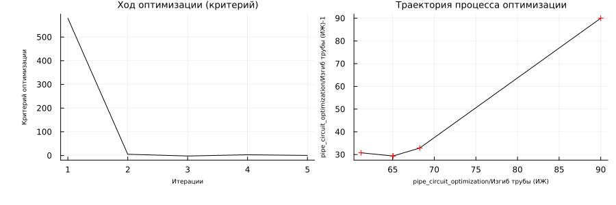
Finally, let's make sure that the search for a solution was really going in the right direction.:
gr()
loss_value = getfield.( result.trace, :value )
xs = first.( trace_point.metadata["x"] for trace_point in Optim.trace(result) );
ys = last.( trace_point.metadata["x"] for trace_point in Optim.trace(result) );
plot(
    plot(loss_value, c=:Black, left_margin=10Plots.mm, bottom_margin=10Plots.mm, xlabel="Iterations", ylabel="Optimization criteria", title="Optimization progress graph (criterion)"),
    plot( xs, ys, c=:Black, markershape=:+, mc=:Red, bottom_margin=10Plots.mm, xlabel=adj.blocks[1], ylabel=adj.blocks[2], title="The trajectory of the optimization process" ),
    leg=false, size=(900,300), guidefont=font(6), titlefont=font(9)
)
Conclusion
We have studied how to wrap a model in a high-level optimization function, and now we can iterate through variables for optimization and select optimizers.