Beamscan and MVDR direction finding algorithms for rectangular headlamps
This example demonstrates the use of the Beamscan and MVDR direction finding algorithms to determine the azimuthal and angular direction of arrival of a signal using a rectangular phased array antenna
Auxiliary functions
# Function for reading data from the `simout` variable
function DataFrame2Array(X)
    squeeze(A) = reshape(A, filter(!=(1), size(A))...)
    out = collect(X)
    out_data = zeros(eltype(out.value[1]),size(out.value[1],1),size(out.value[1],2),length(out.value))
    [out_data[:,:,i] = out.value[i] for i in 1:length(out.value)]

    return squeeze(out_data), out.time
end
function plot_map_doa(X,param,n_step::Int64 = 3;title="",x_lab="Azimuth angle, degrees",
    y_lab="Seat angle, degree",threshold = "auto")
    plotlyjs()
    PARULA_GRAD = cgrad(
        [
            "#352A87", "#0F5CDD", "#127DD8",
            "#079CCF", "#15B1B4", "#59BD8C",
            "#A5BE6B", "#E1B952", "#FCCE2E",
            "#F9FB0E"
    ])
    heatmap(param.RangeAzimuths,param.RangeElevations,X[:,:,n_step],
        color=PARULA_GRAD, title=title,xlabel = x_lab,ylabel=y_lab) |> display;
    return
end
# the function of constructing dynamic visualization of changes in Doppler range and frequency
function calc_matrix_visual(out,param;title_name="")
    gr()
    default(titlefontsize=12,top_margin=5Plots.px,guidefont=10,
        fontfamily = "Computer Modern",colorbar_titlefontsize=8,size=(600,400),
        margin = 2Plots.mm
    )
    PARULA_GRAD = cgrad(
        [
            "#352A87", "#0F5CDD", "#127DD8",
            "#079CCF", "#15B1B4", "#59BD8C",
            "#A5BE6B", "#E1B952", "#FCCE2E",
            "#F9FB0E"
    ])

    x_grid = param.RangeAzimuths
    y_grid = param.RangeElevations

    heatmap(x_grid,y_grid,out[:,:,1],color=PARULA_GRAD,
        xlabel="Azimuth angle, degrees",ylabel="Seat angle, degree",title=title_name,
        colorbartitle="The amplitude")

    @info "Building a visualization of changes in bearing estimates over time..."
    anim1 = @animate for i in axes(out,3)
        mod(i,10)==0 && (@info "$(round(100*i/size(out,3))) %")
        heatmap!(x_grid,y_grid,out[:,:,i],color=PARULA_GRAD)
    end
    @info " , Visualization construction has been completed successfully..."
    return anim1
end;
# Function for running the model
function run_model( name_model, path_to_folder )
    Path = path_to_folder * "/" * name_model * ".engee"
    if name_model in [m.name for m in engee.get_all_models()] # Checking the condition for loading a model into the kernel
        model = engee.open( name_model ) # Open the model
        engee.run( model, verbose=true ); # Launch the model
        engee.close( name_model, force=true ); # Close the model
    else
        model = engee.load( Path, force=true ) # Upload a model
        engee.run( model, verbose=true ); # Launch the model
        engee.close( name_model, force=true ); # Close the model
    end
    return
end;
1. Description of the model structure
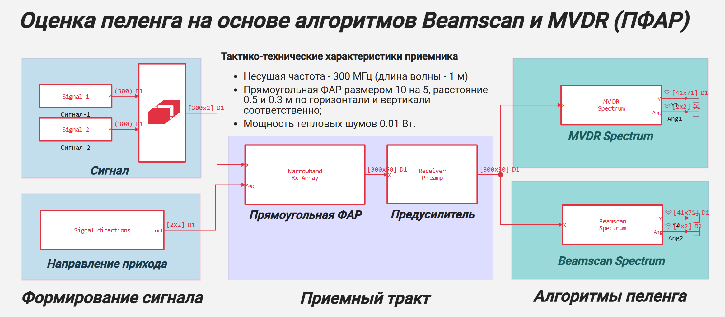
Let's take a closer look at the structural scheme of the model:
Signal generation
This module creates 2 test signals, each of which changes and moves in the azimuthal and angular planes.
- Signal: Implements the signal using a pseudorandom sequence with a normal distribution. In the block, you can set the standard deviation (RMS) of the amplitude, the mathematical expectation and the number of samples in the signal.;
- Reshape: Combines input signals in 2 dimensions;
- Direction of arrival (Signal directions): forms the law of changing the azimuthal and angular direction of arrival of the signal. The output generates a matrix with dimension [2,L], where L is the number of signals.
Receiving path
The subsystem implements the reception and pre-amplification of the incoming signal for a given geometry of a rectangular headlight (in the example [10,5]) taking into account the change in the direction of the signal bearing.
- Rectangular HEADLIGHT (Narrowband Rx Array): used to simulate the reception of a rectangular headlight signal with beam adjustment according to the azimuth-angular direction matrix;
- Amplifier (Receiver Preamp): simulates the passage of a signal through the LNA for a given gain and noise factor (noise temperature) ;
Bearing algorithms
This module directly solves the problem of determining the direction to the target by azimuth and elevation angle using the MVDR Spectrum and Beamscan Spectrum algorithms.
- MVDR Spectrum: Implements a response variance minimization algorithm for calculating the signal bearing;
- Beamscan Spectrum: Implements the spectral analysis algorithm of the scanning beam to calculate the bearing of the signal.
The general block diagram of the system direction finding model is given below:
2. Model operation scenario and initialization of input parameters
To initialize the input parameters of the model, connect the configuration file "Param2DBeamscanMVDRDOA.jl".
include("$(@__DIR__)/Param2DBeamscanMVDRDOA.jl");
In this example, 2 signal sources with different motion scenarios are used - bearing changes:
- source-1 is moving from [30° ** az., 10° places.] in [50° ** az., -5° places.]
- source-2 (with a lower power of 3 dB) is moving from [50° ** az., -5° places.] in [30° ** az., 10° places.]
The scan range is set to -10:60 in azimuth and -20:20 in elevation.
If you need to change the parameter values, then open this file, edit the necessary parameters and save the changes. If the parameters are updated, the following message will be displayed: "The parameters have been initialized successfully!". Otherwise, check the correctness of the changes made to the configuration file.
3. Launching the model
Let's run the simulation of the model using the previously initialized run_model function.:
run_model("2DBeamscanMVDRDOA", @__DIR__);
As soon as the dialog information reads "Progress 100%", it means that the model has worked successfully.
4. Reading the output data
The simulation results for the programmed outputs are written to the "simout" variable. Let's use the DF2Arr function to read the data at the output of the direction finding algorithms.:
sim = collect(simout) # extracting the vector of pledged variables
Ang1,_ = DataFrame2Array(sim[1]) # The resulting output direction of the MVDR algorithm
Ang2,_ = DataFrame2Array(sim[4])  # The resulting direction in the output of the Beamscan algorithm
Y1,_ = DataFrame2Array(sim[2]) # The response map at the output of the MVDR algorithm
Y2,_ = DataFrame2Array(sim[3]);  # The response map of the Beamscan algorithm output
Next, using the plot_map_doa function, we visualize the result of the algorithms for a given modeling step.:
n_step =3 # simulation step number
plot_map_doa(Y1,param2DBeamscanMVDRDOA,n_step;
    title="The result of MVDR Spectrum operation at the $(n_step) modeling step"
)
n_step = 3 # simulation step number
plot_map_doa(Y2,param2DBeamscanMVDRDOA,n_step;
    title="The result of the BeamScan Spectrum operation at the $(n_step) modeling step"
)
5. Animation of simulation results
To create an animation of the algorithms, we use the "cacl_matrix_visual" function, which generates a set of images saved in video format with an extension.gif:
# The MVDR Spectrum Alglorithm
anim1 = calc_matrix_visual(Y1,param2DBeamscanMVDRDOA;title_name="The result of MVDR Spectrum operation")
gif(anim1, "Visual_MVDR.gif", fps = 10);
As a result, a file with the gif extension will be added to the file browser of the current directory.

The animation result for MVDR is shown below:
Similarly, we calculate the dynamic animation for the result of the BeamScan Spectrum algorithm.:
# BeamScan Spectrum Alglorithm
anim2 = calc_matrix_visual(Y2,param2DBeamscanMVDRDOA;title_name="The result of the BeamScan Spectrum")
gif(anim2, "Visual_BeamScan.gif", fps = 10);
Analyzing the obtained graphs, it can be noted that the MVDRSpectrum* algorithm has a higher resolution relative to BeamScan Spectrum: when approaching targets when the distance between them is less than the beam width, their direction of arrival cannot be accurately determined using the beam scanning method. At the same time, the MVDRSpectrum* algorithm greatly weakens the signal in the event of even a slight deviation from the target direction, therefore, "flickering" of targets on the angle diagram is observed.
Conclusion
Thus, in the example, the modeling of the receiving path with an angular coordinate processing unit was considered and a comparative analysis of the MVDR Spectrum and BeamScan Spectrum direction finding algorithms was carried out.
The simulation results showed the advantages and disadvantages of these algorithms:
- MVDR Spectrum - it is advisable to use when the directions of arrival of the signal are known with good accuracy because it has a high resolution;
- Beamscan Spectrum - applicable in case of increased requirements for target detection because it has better noise immunity, inferior resolution.