Localization of targets based on passive radars
This example shows how to simulate the operation scenario of passive radar systems (radars) and determine estimates of the time difference in signal propagation delays (TDOA). to solve the problem of localization in the presence of a large target (aircraft).
This example is the second part of a series of localization solutions. The first part is devoted to the active radar method using the TOA (Time Of Arrival) algorithm for localization of small objects.
Introduction
In the field of radar, the task of locating targets based on data obtained from a group of spatially spaced sensors with known coordinates is of considerable relevance. To solve this problem, methods based on measurements of arrival time (TOA — Time Of Arrival) and arrival time difference (TDOA — Time Difference Of Arrival) of signals are traditionally used.
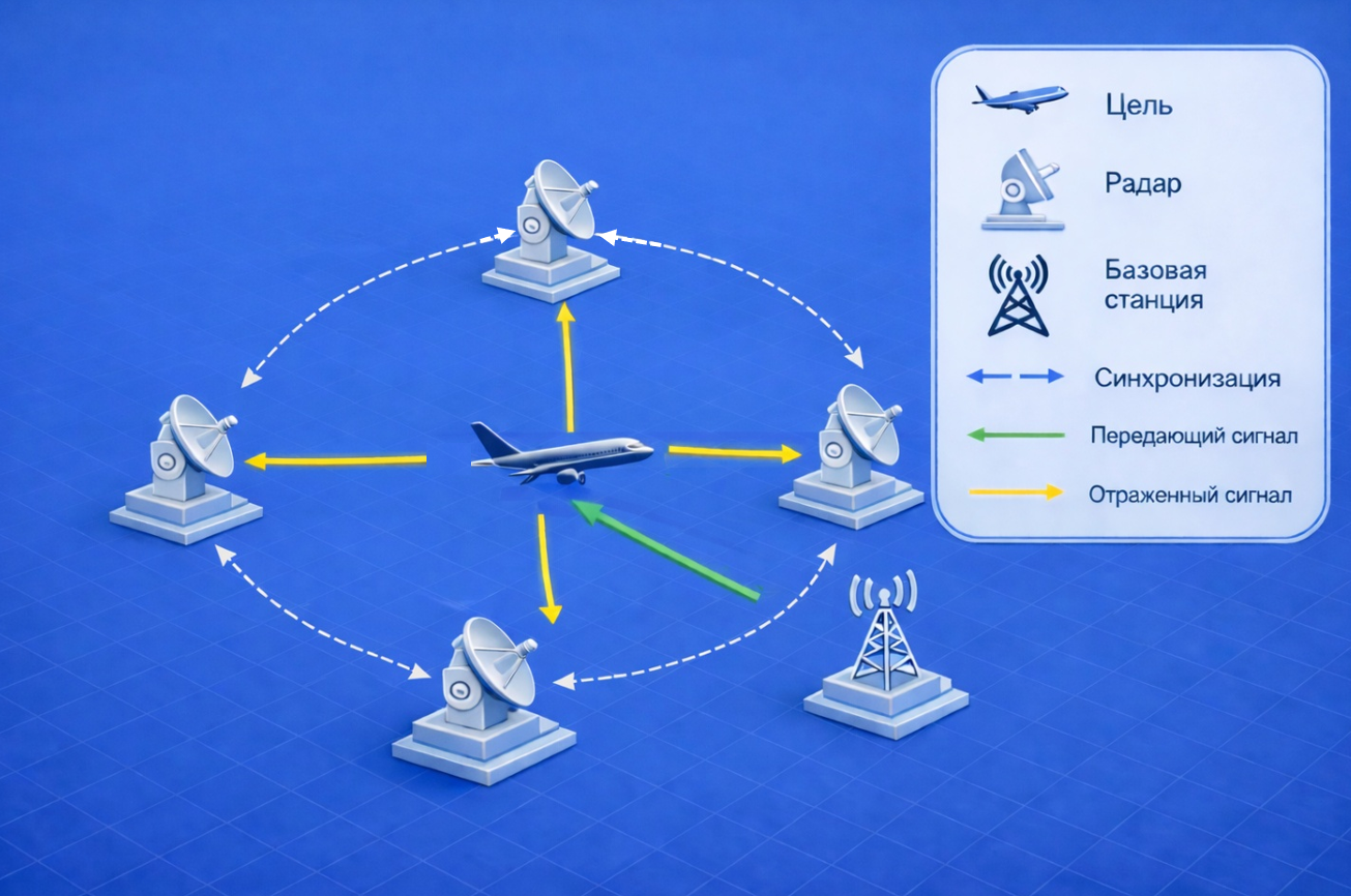
When using the TDOA method A multi-position passive radar system must be used. In this configuration, the target is irradiated by a separate transmission source (base station), and synchronized and distributed radars passively receive reflected signals (see figure below).
In such a system, the type of probing signal is considered unknown. At the same time, other radar stations, cellular base stations, television broadcasting towers, and other similar facilities can act as a transmission source for a passive radar system.
Enabling auxiliary functions
We will perform initialization of the functions necessary for calculating the estimates of positioning and visualization of localization methods TOA/TDOA
isdefined(Main,:init_func) || include("init.jl")
1. Formation of the radar operation scenario
Let's consider using 5 ground-based radar receivers with known locations to locate an aviation target by backscattering signals from a separate tower of an asynchronous transmitter operating in the Ku band.
# Radar Parameters
fc = 12e9 # Hz, carrier frequency
c = physconst("LightSpeed") # m/s, the speed of signal propagation
bw = 100e6 # Hz, signal band
fs = bw # Hz, sampling rate

# Parameters of the receiving and transmitting path
Pt = 10 # W, peak power
Gtx = 40 # dB, gain of the transmitting antenna
Grx = 40 # dB, gain of the receiving antenna
NF = 2.9 # dB, the noise coefficient of the receiving path

# Formation of system objects (CO) of functional radar nodes
antenna = EngeePhased.IsotropicAntennaElement( # WITH an isotropic antenna element
    BackBaffled=false # taking into account the backscattering of the antenna bottom
)
transmitter = EngeePhased.Transmitter( # CO - transmitter
    Gain=Gtx, # transmitter gain
    PeakPower=Pt # Peak power
)
radiator = EngeePhased.Radiator( # CO - transmitting antenna
    Sensor=antenna, # The bottom of the antenna element
    OperatingFrequency=fc # antenna carrier frequency
)
collector = EngeePhased.Collector( # CO - receiving antenna
    Sensor=antenna, # The bottom of the antenna element
    OperatingFrequency=fc # antenna carrier frequency
)
receiver = EngeePhased.ReceiverPreamp(
    Gain=Grx, # receiver gain
    NoiseFigure=NF, # the noise factor in the path
    SampleRate=fs # sampling rate
)

# Creating a CO - goal
tgtrcs = 1000 # m^2, EPR goals
target = EngeePhased.RadarTarget(
    MeanRCS=tgtrcs, # the average EPR value
    PropagationSpeed=c, # The speed of propagation
    OperatingFrequency=fc # ZS carrier frequency
)

# The model of the goal movement scenario
tgtpos = [80; 40; 110]; # [pos_x,pos_y,pos_z],m is the initial position vector
tgtvel = [50; 40; 0]; # [v_x,v_y,v_z],m/s velocity vector
tgtplatform = EngeePhased.Platform( # CO - model of movement
    InitialPosition=tgtpos,  # initial position vector
    Velocity=tgtvel # velocity vector
)

# Radar motion scenario model
radarpos = [ # m, initial positions
    0 300 100 200 150;
    0 50 -200 300 100;
    0 -10 10 5 20
]

# Radar motion scenario model
numRadar = size(radarpos,2) # Number of radars
radarvel = zeros(3,numRadar) # [v_x,v_y,v_z] [m/s], velocity vectors
radarplatform = EngeePhased.Platform( # CO - model of radar movement
    InitialPosition=radarpos,  # initial position vector
    Velocity=radarvel # velocity vector
);

# Base station model
txpos = [-150; -100; 50] # starting position
txvel = [0; 0; 0] # velocity vector
txplatform = EngeePhased.Platform(
    InitialPosition=txpos,
    Velocity=txvel
);
2. Formation of a phasecode manipulation (FCM)
FKM signals is another type of radar signal. Several phase codes can be used in the phase code signal, for example, the code "Zadoff — Chu", the code "Barker", etc. Let's use the code "Zadoff — Chu", the formation of which is implemented using a system object. EngeePhased.PhaseCodedWaveform:
# Formation of a phase-modulated signal
N = 1024 # !!!Number of reports per pulse (fast time counts)
M = 8 # Number of pulses (slow time counts)
numChip = 2^nextpow2(N)-1 # Number of chips in the FKM signal code
tchip = 1/bw # s, the duration of the chip
tWave = numChip * tchip # The modulation period
prf = 1/tWave # Hz, pulse repetition rate

# Configure the phase coded waveform as the maximum length sequence
pmcwWaveform = EngeePhased.PhaseCodedWaveform(
    Code="ZadoffChu", # The signal code
    SampleRate=fs, # sampling rate
    NumChips=numChip, # number of chips
    ChipWidth=tchip, # chip duration
    OutputFormat="Samples", # output format - samples
    NumSamples=numChip  # number of chips per pulse
)
sig_pmcw = pmcwWaveform()*ones(1,M);
println("Dimension of the CC: $(size(sig_pmcw))")
plot_sig_and_spec(sig_pmcw[:,1];fs=fs,name_sig = "FKM")
3. Distribution channel
Since in the current scenario, radars operate in passive mode, therefore, consideration of bidirectional propagation is not required. Let's create a model of the distribution environment for the base station and receiving radars.:
 # the channel model for the base station
txchannel = EngeePhased.FreeSpace(
    PropagationSpeed=c,
    OperatingFrequency=fc,
    SampleRate=fs,
    TwoWayPropagation=false
)

# A similar model for the target-RADAR channel
rxchannel = deepcopy(txchannel);
4. Calculation of the operation scenario of the passive radar system
As in the previous scenario, we will simulate the operation scenario of passive radars using system objects and calculate the reflected signal for each radar in a variable X
# Allocation of memory for the reflected signal for all radars
X = zeros(ComplexF64,size(sig_pmcw)...,numRadar)

# Base station signal
txsig = transmitter.(sig_pmcw)

for rad_i in 1:numRadar
    # Memory allocation for calculating the response from the I-th radar
    x = zeros(ComplexF64,size(sig_pmcw)...)

    # Scenario Model
    for m in 1:M
        # Updates to the position of the base station, radar, and target
        tx_pos,tx_vel = txplatform(tWave)
        radar_pos,radar_vel = radarplatform(tWave)
        tgt_pos,tgt_vel = tgtplatform(tWave)

        # Calculating the viewing angle of the target base station
        _,txang = rangeangle(tgt_pos,tx_pos)

        # radiation from the base station on Wednesday
        radtxsig = radiator(txsig[:,m],txang)

        # Signal propagation from the base station to the target
        txchansig = txchannel(radtxsig,tx_pos,tgt_pos,tx_vel,tgt_vel)

        # Reflection of the signal from the target
        tgtsig = target(txchansig)

        # Signal propagation from the target to the I-th radar
        rxchansig = rxchannel(
            tgtsig,radar_pos[:,rad_i],tgt_pos,
            radar_vel[:,rad_i],tgt_vel
        )

        # Calculating the angle of sight of the radar target
        _,rxang = rangeangle(radar_pos[:,rad_i],tgt_pos)

        # Reception of the reflected signal of the I-th radar
        rxsig = collector(rxchansig,rxang)

        # pre-amplification of the received signal
        x[:,m] .= receiver(rxsig)
    end

    # recording of the received I-th radar signal
    X[:,:,rad_i] .= x

    # Reset the position of the base station, radar and target
    reset_plt!(txplatform,txpos)
    reset_plt!(radarplatform,radarpos)
    reset_plt!(tgtplatform,tgtpos)
end
5. Calculation of delay estimates using the TDOA method
Having calculated the reflected signal of a multi-position passive radar, we will form delay measurements using the TDOA method. Let's use the object TDOAEstimator to evaluate TDOA between different pairs of radars based on the generalized cross-correlation algorithm (GCC) with phase transformation (PHAT).
# Creating a TDOAEstimator object
tdoaEstimator = TDOAEstimator(
    SampleRateSource="Input port", # Sampling rate method (input port)
    VarianceOutputPort=true
)

# Calculation of estimates and variance of delays
Y2, tdoa_var_2 = tdoaEstimator(X, fs);
println("Delay estimates for each pair of radars: $(round.(Y2.*1e9;sigdigits=6)) ns")
SPM analysis of the reflected signal can help us better understand how accurately TDOA is estimated for each pair of radars. We will display the results of the TDOA assessment for a pair of radars using the function plotTDOASpectrum.
plotTDOASpectrum(tdoaEstimator;
    AnchorPairIndex=1:4, # Radar pair numbers
    MaxDelay=1000e-9, # Maximum delay
    DinRange=60, # Dynamic range
    OneSidedSpectrum=false # building a one-way spectrum
)
Having obtained the estimates, the variance of the delay estimates and the known coordinates of the radar, we use the function tdoaposest to determine the location:
tgtposest = tdoaposest(Y2,tdoa_var_2,radarpos)

println("Evaluation of the positions of $(round.(tgtposest;sigdigits=6)) m")
println("The true position of $(tgtpos) m")
Below is a visualization of the localization process using the TDOA method.:
helperPlotTDOAPositions(c,Y2,tgtposest,radarpos,tgtpos,txpos)
Also, we will check the accuracy of location determination using the function RMSE:
RMSE = rmse(tgtposest,tgtpos)
println("Positioning time: $(round(RMSE;sigdigits=6)) m")
Conclusion
The example demonstrates the solution to the problem of locating a target with a passive multi-position radar in the [Engee] simulation environment (https://start.engee.com /). .
This system is a multi-position passive radar system that analyzes phase-coded signals. To solve the positioning problem, algorithms for estimating the time difference in delays (TDOA) were used, followed by localization of the target using the functions TDOAEstimator and tdoaPosest.