Localization of targets based on active radars
This example shows how to simulate the scenario of active radar systems (radars) and determine estimates of the signal propagation delay time (TOA) to solve the localization problem in the presence of a small target.
This example is the first part of a series of localization solutions. The second part is devoted to the passive radar method using the TDOA (Time Difference Of Arrival) algorithm for localization самолета.
Introduction
In the field of radar, the task of locating targets based on data obtained from a group of spatially spaced sensors with known coordinates is of considerable relevance. To solve this problem, methods based on measurements of arrival time (TOA — Time Of Arrival) and arrival time difference (TDOA — Time Difference Of Arrival) of signals are traditionally used.
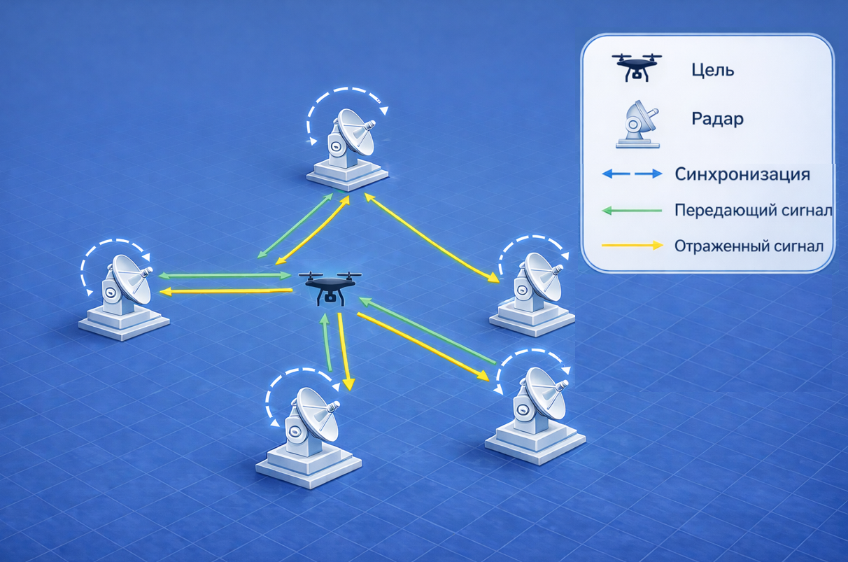
Local positioning of targets using radar can be implemented in various configurations. One of the most common configurations is a monostatic active radar system, which determines the location of a target by actively transmitting radar signals and then receiving reflected signals using a combined and synchronized transmitter and receiver (see figure below).
In such a radar system, TOA is determined based on signal propagation delays between the target and the radar transceiver.
Enabling auxiliary functions
We will perform initialization of the functions necessary for calculating the estimates of positioning and visualization of localization methods TOA
Pkg.add("DSP")
isdefined(Main,:init_func) || include("init.jl")
Consider the localization (TOA) of a target based on a system of monostatic active radars. Each of the radars has a synchronized receiver and transmitter.
1. Formation of the radar operation scenario
Let's create a scenario for the operation of 5 X-band radars with known coordinates to locate an unmanned aerial vehicle (UAV) with a small effective scattering area (ESR).
# Radar Parameters
fc = 9e9 # [Hz], carrier frequency
c = physconst("LightSpeed") # [m/s], the propagation speed of the signal
bw = 200e6 # Hz, signal band
fs = bw # Hz, sampling rate

# Parameters of the receiving and transmitting path
Pt = 1 # W, peak power
Gtx = 40 # dB, gain of the transmitting antenna
Grx = 40 # dB, gain of the receiving antenna
NF = 2.9 # dB, the noise coefficient of the receiving path

# Formation of system objects (CO) of functional radar nodes
antenna = EngeePhased.IsotropicAntennaElement( # WITH an isotropic antenna element
    BackBaffled=false # taking into account the backscattering of the antenna bottom
)
transmitter = EngeePhased.Transmitter( # CO - transmitter
    Gain=Gtx, # transmitter gain
    PeakPower=Pt # Peak power
)
radiator = EngeePhased.Radiator( # CO - transmitting antenna
    Sensor=antenna, # The bottom of the antenna element
    OperatingFrequency=fc # antenna carrier frequency
)
collector = EngeePhased.Collector( # CO - receiving antenna
    Sensor=antenna, # The bottom of the antenna element
    OperatingFrequency=fc # antenna carrier frequency
)
receiver = EngeePhased.ReceiverPreamp(
    Gain=Grx, # receiver gain
    NoiseFigure=NF, # the noise factor in the path
    SampleRate=fs # sampling rate
)

# Creating a CO - goal
tgtrcs = 1e-2 # m^2, EPR goals
target = EngeePhased.RadarTarget(
    MeanRCS=tgtrcs, # the average EPR value
    PropagationSpeed=c, # signal propagation speed
    OperatingFrequency=fc # carrier frequency of the signal
)

# The model of the goal movement scenario
tgtpos = [30; 10; 15]; # [pos_x,pos_y,pos_z],m is the initial vector of the target position
tgtvel = [5; 10; 0]; # [v_x,v_y,v_z],m/s target velocity vector
tgtplatform = EngeePhased.Platform( # CO - model of goal movement
    InitialPosition=tgtpos,  # the initial vector of the target position
    Velocity=tgtvel # The target's velocity vector
)

# Radar motion scenario model
radarpos = [   # m, the initial positions of the radar
    0 -30. 100 80 -40;
    0 50 -40 30 -20;
    0 -5 7 5 2
]
numRadar = size(radarpos,2) # Number of radars
radarvel = zeros(3,numRadar) # [v_x,v_y,v_z] [m/s], radar speeds
radarplatform = EngeePhased.Platform( # CO - model of radar movement
    InitialPosition=radarpos,  # initial position vector
    Velocity=radarvel # Radar speed vector
);
2. Formation of a probing signal (SS)
One of the most popular signals for radar systems is a continuous frequency modulated signal or FMCW signals. FMCW signals are widely used in radar systems, as this method is well-developed and does not require high costs.
# Formation of a continuous signal from the LCHM
N = 1024 # number of counts per rise time (fast time counts )
M = 8 # number of accumulation pulses (slow time counts)
freqSpacing = bw/N # Hz, frequency resolution
tWave = N/fs; # c, the rise time of the saw (pulse duration)
fmcwWaveform = EngeePhased.FMCWWaveform(  # the FMCWWaveform system object
    SweepTime=tWave, # pulse duration
    SweepBandwidth=bw, # signal band (spectrum width)
    SampleRate=fs, # sampling rate
    SweepDirection="Up" # direction of frequency change
)

# Simulation of a continuous FM signal for M channels
sig_lfm = ComplexF64.(fmcwWaveform()*ones(1,M))
println("Dimension of the CC: $(size(sig_lfm))")
Apply the function plot_sig_and_spec for plotting an oscillogram and a spectrogram of a continuous signal with an FM:
plot_sig_and_spec(sig_lfm[:,1];fs=fs,name_sig = "continuous LCHM")
On the spectrogram, it is possible to observe a frequency change from 0 to 200 MHz in 5 microseconds, which meets the specified frequency deviation requirements. `bw` and pulse duration `tWave` The generator
3. Distribution channel
In the scenario under consideration, the model of the signal propagation channel is the free space between each radar and the target in the absence of mutual, passive and active radar interference. To implement the model, we will use the system object EngeePhased.FreeSpace, which allows for attenuation during propagation at the carrier frequency, Doppler shift in the presence of relative motion of the target, and bidirectional propagation (to the target and back).
# Formation of a signal propagation channel taking into account bidirectional propagation
channel = EngeePhased.FreeSpace( # Channel CO-model (free space)
    PropagationSpeed=c, # The speed of propagation
    OperatingFrequency=fc, # carrier frequency
    SampleRate=fs, # sampling rate
    TwoWayPropagation=true # accounting for bidirectional propagation
)
4. Calculation of the scenario of the active radar system
After initializing the system objects necessary to calculate the system operation scenario, we will calculate the reflected signal from the UAV for each radar. The total reflected signal will be stored in a variable
Xwith dimension [N,M,R]:
N is the number of counts in fast time,
M is the number of pulses in slow time.
R is the number of radars in the active system.
# Creating a reference signal
refsig = deepcopy(sig_lfm[:,1])

# Allocation of memory for the reflected signal for all radars
X = zeros(ComplexF64,size(sig_lfm)...,numRadar)

# The signal after the transmitter
txsig = transmitter.(sig_lfm)

for rad_i in 1:numRadar
    # Initializing the input signal
    x = zeros(ComplexF64,size(sig_lfm))

    # Receiving and transmitting path
    for m in 1:M
        # Updating the position of the target and radar
        radar_pos,radar_vel = radarplatform(tWave)
        tgt_pos,tgt_vel = tgtplatform(tWave)

        # Calculation of the bearing angles of the transmitting device
        _,txang = rangeangle(tgt_pos,radar_pos[:,rad_i])

        # The radiation of ZS into space
        radtxsig = radiator(txsig[:,m],txang)

        # Signal propagation in space
        chansig = channel(
            radtxsig,radar_pos[:,rad_i],
            tgt_pos,radar_vel[:,rad_i],tgt_vel
        )

        # Reflection of the signal from the target
        tgtsig = target(chansig)

        # Calculation of the bearing angles of the receiving device
        _,rxang = rangeangle(radar_pos[:,rad_i],tgt_pos)

        # Reception of the reflected signal by the antenna
        rxsig = collector(tgtsig,rxang)

        # Receiver pre-gain
        x[:,m] .= receiver(rxsig)
    end

    dechirpsig = dechirp(x,refsig)
    X[:,:,rad_i] = conj.(dechirpsig)

    # Resetting the position of the radar and the target to calculate the reflected value for the next radar
    reset_plt!(radarplatform,radarpos)
    reset_plt!(tgtplatform,tgtpos)
end
5. Calculation of signal delay estimates and target localization
After calculating the reflected signal for each radar, the next step is to obtain measurements of the time of arrival of the signal. Let's use the object TOAEstimator to estimate the time of arrival of the signal by configuring Measurement="TOA". The spectral analysis method can be configured both FFT and MUSIC.
spectrumMethod = "FFT"; # @param ["FFT", "MUSIC"]
# Formation of the TOAEstimator object
toaEstimator = TOAEstimator(
    PropagationSpeed=c, # The speed of propagation
    Measurement="TOA", # the local positioning method
    SpectrumMethod=spectrumMethod,  # the spectral method
    VarianceOutputPort=true, # enabling the delay error COEX output
    SpatialSmoothing=ceil(Int64,N/2) # for the MUSIC algorithm
);
Let's call the "toaEstimator" object to calculate the delay vector Y1 and the variance vector var1
# Calculation of delay and variance estimates
Y1,toa_var1 = toaEstimator(X,freqSpacing)
println("Delay estimates for each radar: $(round.(Y1.*1e9;sigdigits=6)) ns")
# Construction of the reflected signal spectrum with conversion to propagation delay
plotTDOASpectrum(
    toaEstimator, # delay calculation object
    anchorIdx=1:5, # Radar numbers to display
    MaxDelay=700e-9, # Limit on the delay axis
    DinRange=30, # Dynamic range of SPM
    OneSidedSpectrum=true # building a one-way spectrum
)
Having obtained estimates of the time of signal passage in one direction, the variance of estimates of the time of signal passage and the known coordinates of the radar, we use the function toaposest to determine the location of the target.
Since the obtained estimates of the signal travel time represent estimates of the signal propagation delay in both directions, we divide the estimates of the signal propagation delay by 2 and the estimates of the signal travel time variances by 4.:
# Bidirectional propagation adjustment
Y_single = Y1 ./ 2 # delay, with
var_single = toa_var1 ./ 4 # variance, c^2

# Calculating the estimate of the target's position
tgtposest = toaposest(Y_single,var_single,radarpos)

println("Evaluation of the positions of $(round.(tgtposest;sigdigits=6)) m")
println("The true position of $(tgtpos) m")
Below is a visualization of the localization process using the TOA method.:
helperPlotTOAPositions(c,Y_single,tgtposest,radarpos,tgtpos)
We can also check the accuracy of the location using the RMS error (RMSE).
# Calculation of the COE positioning
RMSE = rmse(tgtposest,tgtpos)
println("Positioning time: $(round(RMSE;sigdigits=6)) m")
Conclusion
The example demonstrates the solution to the problem of locating a small-sized target using an active multi-position radar in an Engee simulation environment (https://start.engee.com /).
This system is a system of monostatic active radars using a continuous signal with linear frequency modulation (FMCW). Methods for estimating the delay time of signal propagation (TOA) are implemented, followed by localization of the signal source based on the functions TOAEstimator and toaPosest.