Introduction

This demo example is dedicated to the task of segmenting ships on radar images. Such images are highly informative and allow you to observe objects regardless of the time of day and weather conditions, but interpreting the data manually requires a lot of effort and knowledge. The use of neural network methods can significantly speed up processing and improve detection accuracy.

The U-Net architecture with the ResNet-18 backbone was chosen due to its ability to take into account both local details and the global context, which is especially important when working with the sea surface and small objects.

Importing libraries and configuring paths

using Pkg
# Pkg.add("DataLoaders")

using FileIO, Images
using ImageTransformations: imresize, Linear
using ProgressMeter, PyCall
using Printf, Dates
using CUDA
using Flux, Metalhead
using BSON: @save, @load
using Statistics, Printf

Setting paths for training and test data: images and masks

train_dir_imgs  = raw"data/train/imgs"
train_dir_masks = raw"data/train/masks"
test_dir_imgs   = raw"data/test/imgs"
test_dir_masks  = raw"data/test/masks";

Hyperparameters of learning

The size of the input (256,256), the size of the batch, and the learning rate are determined

res = (256, 256)          
batch_size = 2
learning_rate = 1e-3

0.001

Dataset

The ImageDataset class is a structure for storing paths to images and masks.
In the getindex method, the data is loaded, scaled to the desired size, and transformed.

function my_collate(samples)
    xs = first.(samples)
    ys = last.(samples)
    return (cat(xs...; dims=4),  
            cat(ys...; dims=4))   
end

my_collate (generic function with 1 method)

struct ImageDataset
    imgs::Vector{String}
    masks::Vector{String}
end

ImageDataset(folder_imgs::String, folder_masks::String) =
    ImageDataset(readdir(folder_imgs; join=true), readdir(folder_masks; join=true))

function Base.getindex(ds::ImageDataset, i::Int)
    img = Gray.(load(ds.imgs[i]))                 
    img = imresize(img, res; method=Linear())   
    x = Float32.(img)                            
    H, W = size(x)
    x = reshape(x, H, W, 1)                      

    msk = Gray.(load(ds.masks[i]))               
    msk = imresize(msk, res) 
    m = Float32.(msk .> 0)                       


    y = cat(1f0 .- m, m; dims=3)

    return x, y
end

Base.length(ds::ImageDataset) = length(ds.imgs)

train_loader and test_loader are created, which feed data to the model using batch files.

train_data = ImageDataset(train_dir_imgs, train_dir_masks)
test_data  = ImageDataset(test_dir_imgs,  test_dir_masks)

train_loader = Flux.DataLoader(train_data; batchsize=batch_size, collate=my_collate, parallel=false)
test_loader  = Flux.DataLoader(test_data;  batchsize=batch_size, collate=my_collate, parallel=false)

50-element DataLoader(::ImageDataset, batchsize=2, collate=my_collate)
  with first element:
  (256×256×1×2 Array{Float32, 4}, 256×256×2×2 Array{Float32, 4},)

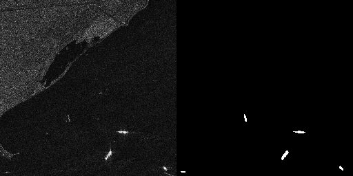
Data visualization

In the cell below, we visualize the data to evaluate what we are working with.

img, mask = train_data[2]

to_rgb(x) = Gray.(dropdims(x; dims=3))

rgb = to_rgb(img)

mask_vis = Gray.(mask[:, :, 2])

hcat(rgb, mask_vis)

Defining the model

UNet is being constructed with the ResNet18 backdoor, the optimizer is being configured (Adam with weight decay), and the GPU is being checked.

model = UNet(res, 1, 2, Metalhead.backbone(Metalhead.ResNet(18; inchannels=1)))

device = CUDA.functional() ? gpu : cpu
model  = device(model)
θ      = Flux.params(model)

opt = Flux.Optimiser(WeightDecay(1e-6), Adam(learning_rate))

Flux.Optimise.Optimiser(Any[WeightDecay(1.0e-6), Adam(0.001, (0.9, 0.999), 1.0e-8, IdDict{Any, Any}())])

Defining training and validation functions

train_step: Makes a forward pass, counts logitcrossentropy, calculates gradients and updates weights.

valid_step: Evaluates the loss based on the validation data.

function train_step(model, θ, x, y, opt)
    loss_cpu = 0f0
    ∇ = Flux.gradient(θ) do
        ŷ = model(x)                              
        l = Flux.logitcrossentropy(ŷ, y; dims=3)
        loss_cpu = cpu(l)
        l
    end
    Flux.Optimise.update!(opt, θ, ∇)
    return loss_cpu
end

function valid_step(model, x, y)
    ŷ = model(x)
    l = Flux.logitcrossentropy(ŷ, y; dims=3)
    return float(l)
end

valid_step (generic function with 1 method)

Model training

The main training cycle of the model is described here. Initially, we set the number of epochs we need.

mkdir("model");

epochs = 50
for epoch in 1:epochs
    println("epoch: ", epoch)
    trainmode!(model)

    train_loss = 0f0
    for (x, y) in train_loader
        train_loss += train_step(model, θ, device(x), device(y), opt)
    end
    train_loss /= length(train_loader)
    @info "Epoch $epoch | Train Loss $train_loss"

    testmode!(model)
    validation_loss = 0f0
    for (x, y) in test_loader
        validation_loss += valid_step(model, device(x), device(y))
    end
    validation_loss /= length(test_loader)
    @info "Epoch $epoch | Validation Loss $validation_loss"

    # saving a checkpoint
    fn = joinpath("model", @sprintf("model_epoch_%03d.bson", epoch))
    @save fn model
    @info "  , the model is saved in $fn"
end

Saving the final model

After training, the model is transferred to the CPU and stored separately in the model1.bson file.

model = cpu(model)
best_path = joinpath("model", "model1.bson")
@info "Saving the model in $best_path"
@save best_path model

[ Info: Сохраняем модель в model/model1.bson

Inference

Auxiliary functions for inference

ship_probs: Extracts the probability of the "ship" class from the network output.

predict_mask: Returns a binary mask or probability map based on the input image.

save_prediction: Saves the predicted mask as a picture.

sci_thresholes: helps you select a threshold for binarization by displaying statistics on different values.

model_on_gpu(m) = any(x -> x isa CuArray, Flux.params(m))
to_dev(x, m)    = model_on_gpu(m) ? gpu(x) : x

function ship_probs(ŷ)
    sz = size(ŷ)
    if sz[3] == 2                
        p = softmax(ŷ; dims=3)
        return Array(@view p[:, :, 2, 1])
    else sz[1] == 2          
        p = softmax(ŷ; dims=1)
        return Array(@view p[2, :, :, 1]) |> x -> permutedims(x, (2,1))
    end
end


function predict_mask(model, img_path; thr=0.35, return_probs=false)
    img = Gray.(load(img_path))
    img = imresize(img, res; method=Linear())
    x = Float32.(img)
    H, W = size(x)
    x = reshape(x, H, W, 1, 1)

    ŷ = model(to_dev(x, model))

    p_ship = ship_probs(ŷ)

    @info "ship prob stats" min=minimum(p_ship) max=maximum(p_ship) mean=mean(p_ship)

    mask = Float32.(p_ship .>= thr)

    return return_probs ? (mask, p_ship) : mask
end

function save_prediction(model, in_path, out_path; thr=0.35)
    m = predict_mask(model, in_path; thr=thr)
    save(out_path, Gray.(m))
    @info "saved" path=out_path positives=sum(m .> 0)
end

function scan_thresholds(model, img_path; ts=0.10:0.05:0.50)
    _, p = predict_mask(model, img_path; return_probs=true)
    for t in ts
        m = p .>= t
        @printf "thr=%.2f  positives=%6d  max=%.3f  mean=%.3f\n" t count(m) maximum(p) mean(p)
    end
end

scan_thresholds (generic function with 1 method)

A probability map is calculated for the selected SAR image, the threshold is selected, and the final pred_mask.png mask is saved.

img_path = raw"data/train/imgs/P0003_1200_2000_4200_5000.png"

scan_thresholds(model, img_path)


save_prediction(model, img_path, "pred_mask.png"; thr=0.50)

Conclusions

In this paper, the UNet neural network was trained with a backbone as a ResNet for SAR image segmentation. The task is not the easiest, because the ships in the images may be located in an urban environment. To further improve the quality of the model, it is necessary to take a more subtle approach to training