Classification of radar signals using deep learning
Introduction
This example shows how to classify radar signals using deep learning.
Modulation classification is an important function of an intelligent receiver. Modulation classification has many applications, for example, in cognitive radars and software-defined radio systems. As a rule, to identify these signals and classify them by type of modulation, it is necessary to identify significant features and enter them into the classifier. This example discusses the automatic extraction of time-frequency features from signals and their classification using a deep learning network.
The first part of this example models a radar signal classification system that synthesizes three pulse signals and classifies them. The waveform of radar signals:
-
Rectangular
-
Linear Frequency Modulation (LFM)
-
Barker's Code
Preparation
Installing the necessary packages
include("PackagesHelper.jl")
using Pkg
Pkg.instantiate()
using CategoricalArrays
using OneHotArrays
using BSON: @save, @load
using Random, Statistics, FFTW, DSP, Images, ImageIO, ImageTransformations, FileIO
using Flux, Metalhead, MLUtils, CUDA, StatsBase, StatisticalMeasures
include("utils.jl");
We will set certain constants related to the device on which the model will be trained, the resolution of images, parameters for data generation, and so on.
Random.seed!(42)
device == gpu ? model = gpu(model) : nothing;
IMG_SZ=(224,224)
OUT="tfd_db"
radar_classes=["Barker","LFM","Rect"]
CLASSES = 1 : length(radar_classes)
N_PER_CLASS=600
train_ratio,val_ratio,test_ratio = 0.8,0.1,0.1
DATA_MEAN=(0.485f0,0.456f0,0.406f0)
DATA_STD=(0.229f0,0.224f0,0.225f0)
We will generate a data set that represents three types of signals. Function helperGenerateRadarWaveforms creates a synthetic dataset of radio signals of three types of modulation: rectangular pulses, LFM chirps and Barker codes. For each signal, parameters (carrier, band, length, modulation direction, etc.) are randomly selected, after which noise, frequency shift, and distortion are added to it. At the output, the function returns a list of complex sequences and a list of labels with the type of modulation for each signal.
data, truth = helperGenerateRadarWaveforms(Fs=1e8, nSignalsPerMod=3000, seed=0)
Next, we turn a set of radio signals into images for subsequent training of the neural network. First, the function tfd_image_gray builds a spectrogram of the signal, converts it to a logarithmic scale, normalizes the values and forms a grayscale image. Then the function save_dataset_as_tfd_images_splits It takes a list of signals and their class labels, randomly divides them into training, validation, and test parts, creates the desired folder structure, and saves the corresponding PNG image of the spectrogram for each signal.
save_dataset_as_tfd_images_splits(data, truth; Fs=1e8, outdir="tfd_db", img_sz=(224,224), ratios=(0.8,0.1,0.1), seed=0)
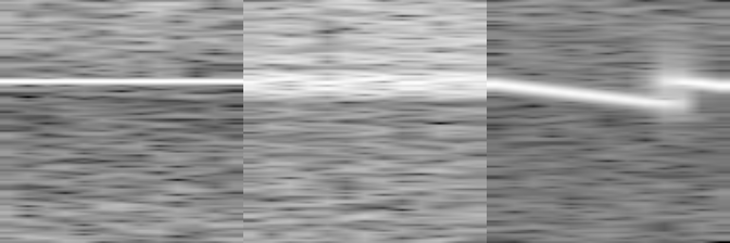
We visualize one signal of each type.
img1 = Images.load(raw"tfd_db/val/Rect/4283146180.png")
img2 = Images.load(raw"tfd_db/val/Barker/3375303598.png")
img3 = Images.load(raw"tfd_db/val/LFM/3736510008.png")
[img1 img2 img3]
Next, we describe the structure that defines the dataset for training the model. Function create_dataset accepts image paths, loads them into memory, and then applies transformations to them, such as resizing and rearranging axes in the order required by FLux.
function Augment_func(img)
    resized = imresize(img, 224, 224)
    rgb = RGB.(resized)
    ch = channelview(rgb)
    x = permutedims(ch, (3,2,1))
    Float32.(x)
end
function Create_dataset(path)
    img_train = []
    img_test = []
    img_valid = []
    label_train = []
    label_test = []
    label_valid = []

    train_path = joinpath(path, "train");
    test_path = joinpath(path, "test");
    valid_path = joinpath(path, "val");

    function process_directory(directory, img_array, label_array, label_idx)
        for file in readdir(directory)
            if endswith(file, ".jpg") || endswith(file, ".png")
                file_path = joinpath(directory, file);
                img = Images.load(file_path);
                img = Augment_func(img);
                push!(img_array, img)
                push!(label_array, label_idx)
            end
        end
    end


    for (idx, label) in enumerate(readdir(train_path))
        println("Processing label in train: ", label)
        label_dir = joinpath(train_path, label)
        process_directory(label_dir, img_train, label_train, idx);
    end


    for (idx, label) in enumerate(readdir(test_path))
        println("Processing label in test: ", label)
        label_dir = joinpath(test_path, label)
        process_directory(label_dir, img_test, label_test, idx);
    end

    for (idx, label) in enumerate(readdir(valid_path))
        println("Processing label in valid: ", label)
        label_dir = joinpath(valid_path, label)
        process_directory(label_dir, img_valid, label_valid, idx);
    end

    return img_train, img_test, img_valid, label_train, label_test, label_valid;
end;
Creating a dataset
img_train, img_test, img_valid, label_train, label_test, label_valid = Create_dataset("tfd_db");
Creating data loaders
train_loader = DataLoader((data=img_train, label=label_train), batchsize=64, shuffle=true, collate=true)
test_loader = DataLoader((data=img_test, label=label_test), batchsize=64, shuffle=false, collate=true)
valid_loader = DataLoader((data=img_valid, label=label_valid), batchsize=64, shuffle=false, collate=true)
Next, we describe the functions for training and validating the model.
function train!(model, train_loader, opt, loss_fn, device, epoch::Int, num_epochs::Int)
    Flux.trainmode!(model)
    running_loss = 0.0
    n_batches    = 0

    for (data, label) in train_loader
        x  = device(data)
        yoh = Flux.onehotbatch(label, CLASSES) |> device

        loss_val, gs = Flux.withgradient(Flux.params(model)) do
            ŷ = model(x)
            loss_fn(ŷ, yoh)
        end
        Flux.update!(opt, Flux.params(model), gs)

        running_loss += Float64(loss_val)
        n_batches    += 1
    end

    return opt, running_loss / max(n_batches, 1)
end


function validate(model, val_loader, loss_fn, device)
    Flux.testmode!(model)
    running_loss = 0.0
    n_batches    = 0

    for (data, label) in train_loader
        x  = device(data)
        yoh = Flux.onehotbatch(label, CLASSES) |> device

        ŷ = model(x)
        loss_val = loss_fn(ŷ, yoh)

        running_loss += Float64(loss_val)
        n_batches += 1
    end

    Flux.trainmode!(model)
    return running_loss / max(n_batches, 1)
end
Initializing the SqueezeNet model
model = SqueezeNet(pretrain=false, nclasses=length(radar_classes))
model = gpu(model);
Let's set the loss function, the optimizer, and the learning rate.
lr = 0.0001
lossFunction(x, y) = Flux.Losses.logitcrossentropy(x, y);
opt = Flux.Adam(lr, (0.9, 0.99));
Classes = 1:length(radar_classes);
Let's start the training cycle of the model
no_improve_epochs = 0
best_model    = nothing
train_losses = [];
valid_losses = [];
best_val_loss = Inf;
num_epochs = 50
for epoch in 1:num_epochs
    println("-"^50 * "\n")
    println("EPOCH $(epoch):")

    opt, train_loss = train!(
        model, train_loader, opt,
        lossFunction, gpu, 1, num_epochs
    )

    val_loss = validate(model, valid_loader, lossFunction, gpu)

    if val_loss < best_val_loss
        best_val_loss = val_loss
        best_model = deepcopy(model)
    end

    println("Epoch $epoch/$num_epochs | train $(round(train_loss, digits=4)) | val $(round(val_loss, digits=4))")

    push!(train_losses, train_loss)
    push!(valid_losses, val_loss)

end
Saving the trained model
model = cpu(model)
@save "$(@__DIR__)/models/modelCLSRadarSignal.bson" model
Testing the model
Let's perform an inference, and also build an error matrix.
model_data = load("$(@__DIR__)/models/modelCLSRadarSignal.bson")
model = model_data[:model] |> gpu;
Let's write a function to evaluate the trained model, which calculates the Accuracy metric.
total_loss, correct_predictions, total_samples = 0.0, 0, 0
all_preds = []
True_labels = []
for (data, label) in enumerate(test_loader)

    x  = gpu(data)
    yoh = Flux.onehotbatch(label, CLASSES) |> gpu


    ŷ = model(x)
    total_loss= loss_fn(ŷ, yoh)
    # y_pred = model(imgs, feat)
    # total_loss += Flux.Losses.logitcrossentropy(y_pred, onehotbatch(y, classes))
    preds = onecold(ŷ, classes)
    true_classes = y
    append!(all_preds, preds)
    append!(True_labels, true_classes)
    correct_predictions += sum(preds .== true_classes)
    total_samples += length(y)
end

accuracy = 100.0 * correct_predictions / total_samples
accuracy_score, all_preds, true_predS = evaluate_model_accuracy(test_loader, model, CLASSES);
println("Accuracy trained model:", accuracy_score, "%")
We will also test it on a specific object.
classes = readdir("tfd_db/train")
cls = rand(classes)
files = readdir(joinpath("tfd_db/train", cls))
f = rand(files)
path = joinpath("tfd_db/train", cls, f)

img = Images.load(path)
img = Augment_func(img)
img = reshape(img, size(img)..., 1)
ŷ = model(gpu(img))
probs = Flux.softmax(ŷ)
pred_idx = argmax(Array(probs))
pred_class = radar_classes[pred_idx]

println("The true class: ", cls)
println("Predicted class: ", pred_class)
Conclusion
In this demo example, a convolutional neural network was trained to classify radar signals.
The learning outcomes have good indicators