Determining influential features for a random forest model
Introduction
In modern data analysis, the task of predicting continuous quantities occupies a central place in a variety of applied fields, from economics and bioinformatics to automotive engineering and energy. One of the most widely used methods for solving such problems is Random Forest, an ensemble machine learning algorithm proposed by Leo Breiman in 2001.
A random forest is an ensemble of regression trees, each of which is based on an independent sample from the source data. The basic element here is a regression tree, a hierarchical structure of the "decision tree" type, at the nodes of which the feature space is sequentially divided into more homogeneous regions. Ensembling is based on the idea that combining many simple models into a single composition allows for higher accuracy and stability of forecasts than using any of them individually.
A separate problem when building decision trees is the presence of missing values in the data. The surrogate splitting mechanism is used to solve it. When optimal partitioning by the main feature is impossible due to omission, the algorithm automatically selects an alternative feature, the partitioning of which mimics the original one as much as possible.
This example shows a strategy for choosing a partitioning criterion when building a regression random forest. The analysis solves the problem of identifying the key predictors that make the greatest contribution to the predictive ability of the model, which justifies their mandatory inclusion in the final training dataset.
Initial data
We will attach the necessary files and libraries.
# EngeePkg.purge()
# import Pkg
# Pkg.add(["DataFrames", "XLSX", "CategoricalArrays", "MLJ", "MLJDecisionTreeInterface", "StableRNGs", "EvoTrees", "DecisionTree", "Statistics", "Random", "PyPlot"])
using DataFrames, XLSX, CategoricalArrays, MLJ, MLJDecisionTreeInterface, StableRNGs, EvoTrees, DecisionTree, Statistics, Random, PyPlot
foreach(include, filter(contains(r"\.jl$"), readdir()))
A data set containing the characteristics of passenger cars is used for the analysis. As part of the study, a regression model is being built that predicts fuel consumption based on the following parameters:
- number of cylinders;
- Engine displacement;
- Power;
- Vehicle weight;
- Acceleration time;
- year of release;
- Country of origin.
X = XLSX.readdata("автомобили.xlsx", "Sheet1", "A:G")
X = DataFrame(X[2:end, :], Symbol.(X[1, :]))
Download the fuel consumption data.
расход_ = XLSX.readdata("expenditure.xlsx", "Sheet1", "A:A")
Expense = parse.(Float64, flow_[2:end])
There is a lack of fuel consumption data for some vehicles. This will be taken into account in further calculations.
Determining the number of unique feature values
Let's determine the number of unique values of each feature from the dataset.
for column in names(X)
    try
        X[!, column] = [getdata(val) for val in X[!, column]]
    catch e
        X[!, column] = categorical(X[!, column])
    end
end
unique = [length(unique(skipmissing(X[!, column]))) for column in names(X)]
Let's compare the unique values using a bar chart.
graph1 = Plots.bar(1:length(unique), unique,
    title = "Number of unique values",
    ylabel = "Unique values",
    xticks = (1:length(unique), names(X)[1:end]),
    ylims = (0, maximum(unique) * 1.1),
    xrotation = 45,
    legend = false,
    bar_width = 0.7,
    color = :steelblue)
display(graph1)
The diagram shows that there are significant differences in the number of unique feature values. Such a disparity creates the risk of biasing estimates when using a standard algorithm for selecting splitting variables at the nodes of random forest trees, therefore, to form an ensemble of regression trees, it is necessary to take into account the relationship between the features.
Formation of an ensemble of regression trees
To evaluate the indicators of the importance of features, it is necessary to train an ensemble consisting of regression trees, taking into account the relationship between the features. Let's create a training sample.
X_matrix = zeros(Float64, nrow(X), ncol(X))
col_names = names(X)

for (j, col) in enumerate(eachcol(X))
    if eltype(col) <: String || eltype(col) <: CategoricalValue
        unique_vals = unique(col)
        val_to_num = Dict(val => i for (i, val) in enumerate(unique_vals))
        X_matrix[:, j] = [Float64(val_to_num[x]) for x in col]
    else
        X_matrix[:, j] = Float64.(col)
    end
end

train_idx = .!isnan.(Expense)
X_train = X_matrix[train_idx, :]
y_train = Flow rate[train_idx]

println("Training sample size: $(size(X_train, 1)) rows")
println("Number of attributes: $(size(X_train, 2))")
Let's complete the ensemble training.
Random.seed!(1)
trees = 200
trees, yHat_train = build_forest(y_train, X_train, 0, trees, 0.632, -1, 5, 2)
valid_pred_idx = .!isnan.(yHat_train)
if sum(valid_pred_idx) > 0
    R2 = cor(y_train[valid_pred_idx], yHat_train[valid_pred_idx])^2
    println("R² = ", R2)
end
The value of the coefficient of determination This indicates that the model explains 87% of the spread of the target variable relative to the average value.
Evaluation of the attribute's impact
The influence of features is estimated by rearranging out-of-sample observations between the ensemble trees.
importance = permutation_importance(trees, X_train, y_train, 5);
Meaning важность It is a 1×7 vector containing estimates of the influence of the initial features. A feature of the estimates obtained is the absence of bias towards features with a large number of unique values. Let's compare the obtained indicators of the influence of the signs.
graph2 = Plots.bar(importance,
    title = "Indicators of the influence of signs",
    xlabel = "Signs",
    ylabel = "Influence",
    xticks = (1:length(unique), names(X)[1:end]),
    ylims = (0, maximum(importance) * 1.1),
    xrotation = 45,
    legend = false,
    bar_width = 0.7,
    color = :steelblue)
display(graph2)
Higher values of estimates correspond to more influential predictors. According to the bar chart, the year of manufacture of the car has the greatest predictive value, followed by the weight of the car.
Let's display the estimates of the relationship of the features in the form of a color matrix.
график3 = imshow(predAssociation, cmap="viridis", aspect="auto", interpolation="nearest")
title("Evaluation of the relationship of features")
colorbar(label="The relationship")
PyPlot.xticks(0:length(col_names)-1, col_names, rotation=45, ha="right")
PyPlot.yticks(0:length(col_names)-1, col_names)
display(graph3)
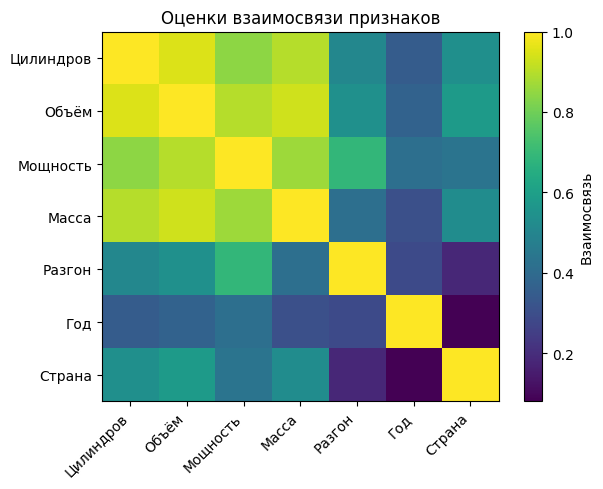
A predictive measure of the relationship is an indicator that characterizes the degree of similarity between the decision rules used to divide observations. The maximum value of this measure is achieved for the best surrogate splitting.
The matrix elements allow us to conclude about the strength of the relationship between the features: higher values indicate a stronger correlation between the corresponding features.
Conclusion
This example demonstrates an approach to building a regression random forest with an emphasis on the correct selection of influential features. Using the example of a set of car characteristics, the problem of predicting fuel consumption is solved — a typical problem for the automotive industry, where the accuracy of the model affects engineering solutions.
The surrogate splitting mechanism made it possible to correctly process data gaps and construct a matrix of feature relationships that provides a meaningful interpretation of the dependency structure in the data.
The presented methodology is universal and applicable in a wide range of fields: from mechanical engineering to bioinformatics. The main practical conclusion is that the correct consideration of the nature of variables when choosing a partitioning criterion makes it possible to increase the accuracy of forecasts and obtain meaningful conclusions about the significance of factors free from statistical biases.