Configuring the neural network learning process
In this example, we will create an environment for training a neural network, controlled using a convenient graphical form.
Task description
The development of neural networks has long ceased to be the domain of researchers with many years of experience in writing code. Today it is a tool for an engineer, analyst, and product scientist. However, the entry threshold is often still high: even for a simple fully connected network with three layers, you need to remember the syntax of libraries like Flux.jl and correctly load the dataset from CSV and output the correct graphs... This is where graphical interfaces (GUIs) come to the rescue. They allow you to focus on the essence of the task — working on data quality and interpretation of the result, rather than on trivial mistakes that everyone makes at the first stage.
Let's create an interface for training a neural network, which will still hide the same mathematics and data operations that load, distribute, train, and check the quality of the neural network.
Preparatory operations include the installation of a library for training neural networks:
# It may take a minute to compile the Flux library.
Pkg.add(["Flux", "Interpolations"])
using Flux, CSV, DataFrames, Random
using Flux: mse
using Statistics, Interpolations
gr()
Now we will develop a GUI that allows you to move the slider and train a neural network with the required number of neurons, which will load data and train the neural network.
Assumptions: the script folder contains the train.csv and test.csv files. The first column of each file contains the predicted variable, the remaining columns contain the attributes. We are solving a regression problem.
# Let's move to the directory with this script.
cd(@__DIR__)
train_filename = "train.csv" # @param {type:"string"}
test_filename = "test.csv" # @param {type:"string"}
train_df = CSV.read(train_filename, DataFrame, types=Float32)
test_df = CSV.read(test_filename, DataFrame, types=Float32)
# We assume that the first column contains the predicted values, and the rest contain the signs
X_train = Matrix(train_df[:, 2:end])' # (n_features, n_samples)
X_test = Matrix(test_df[:, 2:end])' # (n_features, n_samples)
y_train_raw = reshape(train_df[:, 1], 1, :) # (1, n_samples)
y_test_raw = reshape(test_df[:, 1], 1, :) # (1, n_samples)
# Normalization of signs
X_train_mean = mean(X_train, dims=2)
X_train_std = std(X_train, dims=2)
# Normalize train and test with train selection parameters
X_train_norm = (X_train .- X_train_mean) ./ X_train_std
X_test_norm = (X_test .- X_train_mean) ./ X_train_std
# Normalize the target values
y_train_mean = mean(y_train_raw)
y_train_std = std(y_train_raw)
y_train_norm = (y_train_raw .- y_train_mean) ./ y_train_std
y_test_norm = (y_test_raw .- y_train_mean) ./ y_train_std
features_count = size(X_train_norm, 1)
l1_neurons = 30 # @param {type:"slider",min:1,max:30,step:1}
l2_neurons = 28 # @param {type:"slider",min:1,max:30,step:1}
l3_neurons = 25 # @param {type:"slider",min:1,max:30,step:1}
l4_neurons = 13 # @param {type:"slider",min:1,max:30,step:1}
l5_neurons = 1 # @param {type:"slider",min:1,max:30,step:1}
n_epochs = 499 # @param {type:"slider",min:1,max:500,step:1}
# Architecture for regression
model = Chain(
Dense(features_count => l1_neurons, relu),
Dense(l1_neurons => l2_neurons, relu),
Dense(l2_neurons => l3_neurons, relu),
Dense(l3_neurons => l4_neurons, relu),
Dense(l4_neurons => l5_neurons, relu),
Dense(l5_neurons => 1)
)
# Training
loss(m, x, y) = mse(m(x), y)
opt_state = Flux.setup(Adam(0.001), model)
data = [(X_train_norm, y_train_norm)]
train_losses = []
test_losses = []
# Starting the training
for epoch in 1:n_epochs
Flux.train!(loss, model, data, opt_state)
push!(train_losses, loss(model, X_train_norm, y_train_norm))
push!(test_losses, loss(model, X_test_norm, y_test_norm))
end
# Functions for converting between scales
denormalize_y(y_norm) = y_norm .* y_train_std .+ y_train_mean
denormalize_X(X_norm, dim) = X_norm .* X_train_std[dim] .+ X_train_mean[dim]
test_loss = loss(model, X_test_norm, y_test_norm)
println("\nMSE on the test (on a normalized scale): $(round(test_loss, digits=6))")
println("RMSE on the test (in initial units): $(round(sqrt(test_loss) * y_train_std, digits=2))")
# An example of a prediction for the first object from the test
prediction_norm = model(X_test_norm[:, 1:1])
actual_norm = y_test_norm[:, 1:1]
prediction = denormalize_y(prediction_norm)
actual = denormalize_y(actual_norm)
println("Example (normalized): predicted by $(round.(prediction_norm, digits=3)), really $(round.(actual_norm, digits=3))")
println("Example (initial scale): predicted $(round.(prediction, digits=2)), really $(round.(actual, digits=2))")
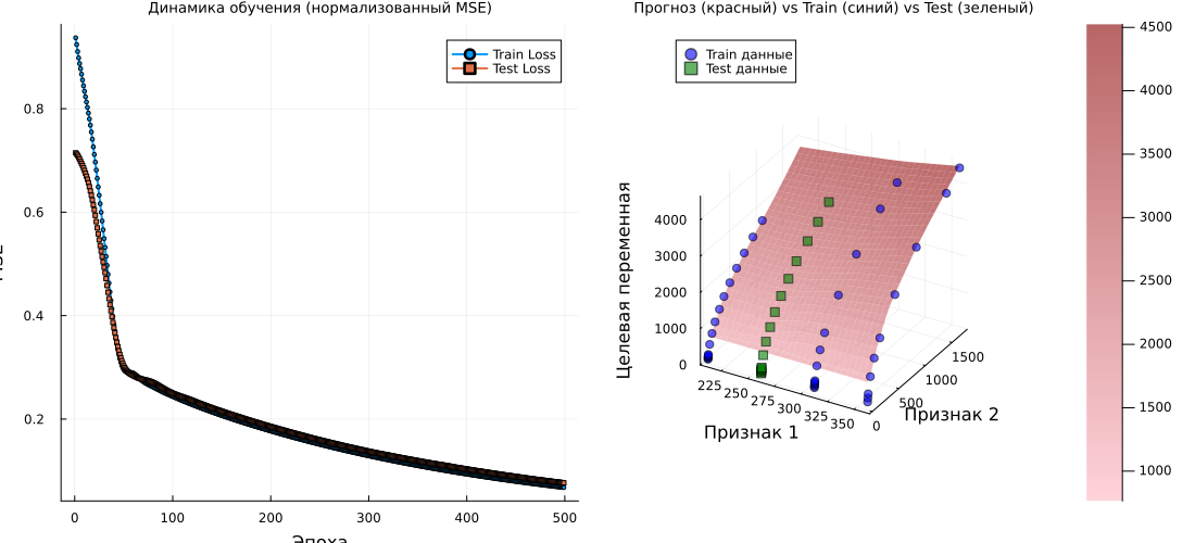
# Graph 1: Learning Curves
p1 = plot(1:n_epochs, train_losses, label="Train Loss", lw=2, marker=:circle, markersize=2)
plot!(p1, 1:n_epochs, test_losses, label="Test Loss", lw=2, marker=:square, markersize=2)
title!(p1, "Learning Dynamics (normalized MSE)")
xlabel!(p1, "Era")
ylabel!(p1, "MSE")
# Graph 2: 3D surface
if features_count >= 2
n_points = 30
# Ranges in a normalized space
x1_range_norm = range(extrema(X_train_norm[1, :])..., length=n_points)
x2_range_norm = range(extrema(X_train_norm[2, :])..., length=n_points)
# Creating a grid in a normalized space
grid_x1_norm = repeat(x1_range_norm', n_points, 1)
grid_x2_norm = repeat(x2_range_norm, 1, n_points)
# For the remaining signs, we take the average values (in a normalized space)
grid_other_norm = zeros(features_count-2, n_points, n_points)
for i in 3:features_count
grid_other_norm[i-2, :, :] .= mean(X_train_norm[i, :])
end
# Creating a complete set of features for the grid (in a normalized space)
grid_points_norm = vcat(
reshape(grid_x1_norm, 1, n_points, n_points),
reshape(grid_x2_norm, 1, n_points, n_points),
grid_other_norm
)
grid_points_flat_norm = reshape(grid_points_norm, features_count, n_points * n_points)
# Predictions of the model on a grid (on a normalized scale)
predictions_norm = model(grid_points_flat_norm)
predictions_2d_norm = reshape(predictions_norm, n_points, n_points)
# Converting the predictions to the original scale for visualization
predictions_2d_original = denormalize_y(predictions_2d_norm)
# Converting the grid coordinates to the original scale for visualization
x1_range_original = denormalize_X(x1_range_norm, 1)
x2_range_original = denormalize_X(x2_range_norm, 2)
# Initial data points (train) in the original scale
X1_train_original = denormalize_X(X_train_norm[1, :], 1)
X2_train_original = denormalize_X(X_train_norm[2, :], 2)
y_train_original = vec(denormalize_y(y_train_norm))
# Test data points in the original scale
X1_test_original = denormalize_X(X_test_norm[1, :], 1)
X2_test_original = denormalize_X(X_test_norm[2, :], 2)
y_test_original = vec(denormalize_y(y_test_norm))
# Prediction surface at the initial scale
p2 = surface(x1_range_original, x2_range_original, predictions_2d_original,
alpha=0.6, label="Neural network forecast",
camera=(30, 30), color=:reds)
# Adding training points (blue)
scatter!(p2, X1_train_original, X2_train_original, y_train_original,
label="Train data",
color=:blue,
markersize=4,
alpha=0.7,
markeralpha=0.6)
# Adding test points (green)
scatter!(p2, X1_test_original, X2_test_original, y_test_original,
label="Test data",
color=:green,
markersize=4,
alpha=0.7,
markeralpha=0.6,
marker=:square)
title!(p2, "Forecast (Red) vs Train (Blue) vs Test (Green)")
xlabel!(p2, "Sign 1")
ylabel!(p2, "Sign 2")
zlabel!(p2, "Target variable")
# # We output statistics for verification
# println("\n Ranges for visualization:")
# println("x1: [$(round(minimum(x1_range_original), digits=2)), $(round(maximum(x1_range_original), digits=2))]")
# println("x2: [$(round(minimum(x2_range_original), digits=2)), $(round(maximum(x2_range_original), digits=2))]")
# println("y(predictions): [$(round(minimum(predictions_2d_original), digits=2)), $(round(maximum(predictions_2d_original), digits=2))]")
# println("y (train): [$(round(minimum(y_train_original), digits=2)), $(round(maximum(y_train_original), digits=2))]")
# println("y (test): [$(round(minimum(y_test_original), digits=2)), $(round(maximum(y_test_original), digits=2))]")
plot(p1, p2, layout=(1, 2), titlefont=font(9), guidesfont=font(7), size=(1100,500))
else
plot(p1, titlefont=font(9), guidesfont=font(7), size=(800,300))
end
Hide the code by double-clicking on the form to enter the parameters.
Check that the cell auto execution enabled (button should be green).
And post the output to the right of the cell, if it is on the bottom. Your toolkit is ready!
Conclusion
The code for this task is concise and solves a specific problem. But since we packaged this functionality into a graphical interface, you just had to select the number of neurons in each layer and see how the quality of the forecast changes.
This is the fastest way to train the first 5-10 neural networks for unknown data and see if this type of model is suitable for your tasks.