Surrogate neural network from a physical model

Let's look at how to create a neural network to replace the physical model, which will allow us to simplify calculations, achieve portability to controllers, or hide implementation details.

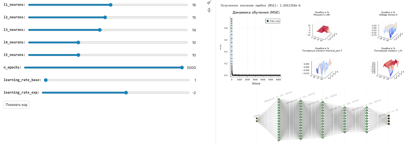
As a result, we can easily change the parameters of the neural network using a masked code cell and check the quality of the forecast according to this schedule.:

Model Conversion

Why might it be necessary to transform the model into a neural network? There may be many scenarios where this is interesting.:

convert the model into code for the controller,
speed up the execution of the model to run it in a loop,
hide the details of the model implementation, leaving only the calculations.

Neural networks are a well-studied and simple form of model assignment, especially fully connected ones, which we will use in this project.

We will install and download several libraries, as well as open a model that we will convert into a neural network.

For this example, we took a model from the [Fuel Cell System] project(https://engee.com/community/ru/catalogs/projects/sistema-toplivnykh-elementov ) the author shestakoviktor.

Pkg.add(["ChainPlots", "Flux"])
using DataFrames, CSV, Flux, Random, Statistics, ChainPlots
using Flux: mse
gr();

engee.open( "$(@__DIR__)/" * "FuelCell.engee");

Our approach will allow us to analyze the results obtained through engee.run() for different input conditions. We will set the conditions by changing the parameters of different blocks using engee.set_param!().

We will not be able to change global variables in the loop, only block properties. Julia does not allow manipulation of global variables inside local procedures. Changing the properties of the blocks leaves less chance that we will forget to make some calculations with global calculations before executing.

Defining interfaces

Our model will have 4 output variables (4 targets in neural network terminology):

out_vars = ["Power kW", "Voltage Sensor.V", "The fuel cell.thermal_port.T", "Fuel cell.i_FC"]

4-element Vector{String}:
 "Мощность кВт"
 "Voltage Sensor.V"
 "Топливный элемент.thermal_port.T"
 "Топливный элемент.i_FC"

All these structures can be set in different ways, for example, setting input variables (two features) via a CSV table.:

csv_text = """
block,                            param,    units,    delta,    lower,     upper
FuelCell/Hydrogen pressure (bar), Value, , 2.0, 2.0, 20.0
FuelCell/Fuel supply, slope, , 10/60, 50/60, 150/60
"""

adj_vars = CSV.read(IOBuffer(csv_text), DataFrame)

And another option is to create dictionaries of parameters and combine them into a DataFrame.:

v1 = Dict(:block=>"FuelCell/Hydrogen Pressure (bar)",:param=>"Value", :units=>"", :delta=>2.0, :lower=>2.0, :upper=>20.0)
v2 = Dict(:block=>"FuelCell/Fuel supply",:param=>"slope", :units=>"", :delta=>10/60, :lower=>50/60, :upper=>150/60)
adj_vars = vcat(DataFrame.([v1, v2])...)

Thus, we have set the number of inputs and outputs of the neural network into which we will turn the physical model.:

n_features, n_targets= nrow(adj_vars), length(out_vars)

(2, 4)

Experiment planning

Let's prepare the table result_df. The number of columns in this table is equal to the number of runs of the original model with different combinations of input parameters. Their range is set in the settings of the input variables (the lower limit lower, the upper limit upper And the step delta).

ranges = [collect(row.lower:row.delta:row.upper) for row in eachrow(adj_vars)]
combinations = collect(Iterators.product(ranges...))

# A table with combinations of values of all ranges from adj_vars
result_df = DataFrame()
for (i, row) in enumerate(eachrow(adj_vars))
    col_name = Symbol("$(row.block)/$(row.param)")
    result_df[!, col_name] = [comb[i] for comb in combinations[:]]
end

println("Number of model launches: ", nrow(result_df))
first( result_df, 4 )

Количество запусков модели: 110

Launching the model

Let's go through all the rows of the experiment table and fill it with the values of the output variables.

As output variables, let's take the final value of each signal we are interested in.

When the data is collected, it is better to comment out this cell.

# Creating new columns for output variables
for var in out_vars result_df[!, Symbol(var)] = fill(Float64(NaN), nrow(result_df)); end

# We set the parameters and run the model
for row in eachrow(result_df)
    for (i, col) in enumerate(names(result_df)[1:end-length(out_vars)])
        block, param, unit = adj_vars.block[i], adj_vars.param[i], adj_vars.units[i]
        unit == "" ? engee.set_param!(block, param => string(row[col])) : engee.set_param!(block, param => Dict("value" => string(row[col]), "unit" => String(unit)));
    end
    data = engee.run()
    for var in out_vars row[Symbol(var)] = length(data[var].value) > 1 ? data[var].value[end] : NaN; end
end

# We will save the results for further processing.
CSV.write("$(@__DIR__)/data/outputfile.csv", result_df)
first( result_df, 4 )

We can see that some of the launches ended unsuccessfully. In these places, the output parameters are NaN. The reason is incompatible input parameter values or solver settings that can be improved.

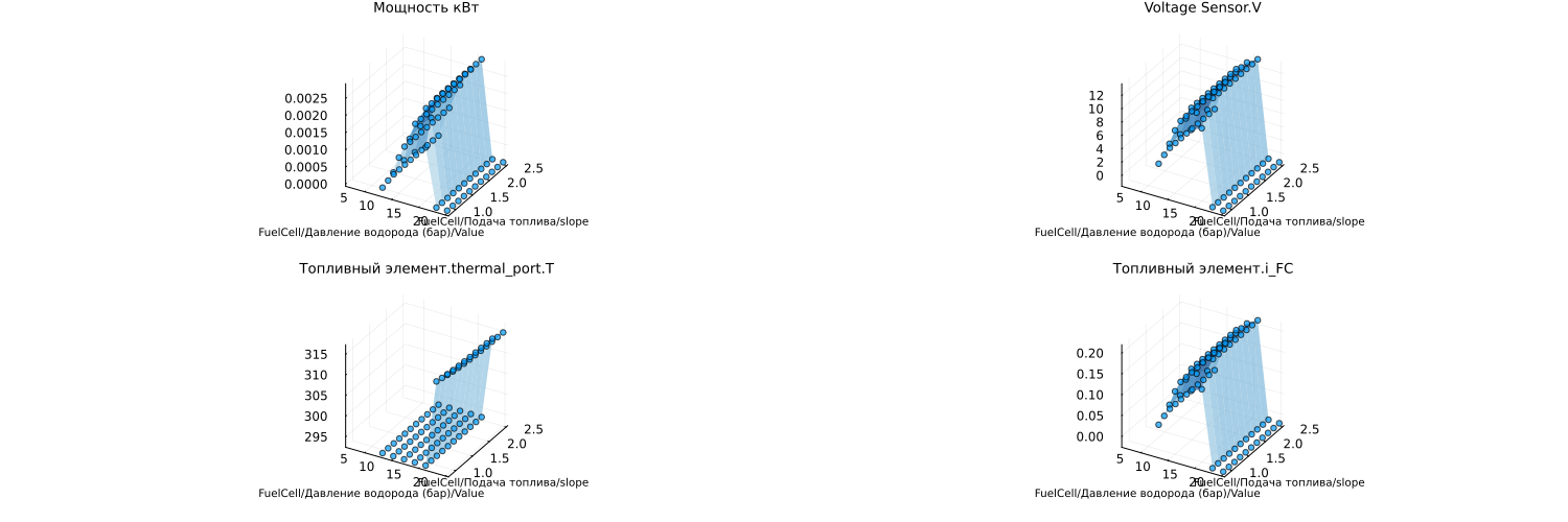
Here are the graphs that we will reproduce using a neural network.:

result_df = DataFrame(CSV.File("$(@__DIR__)/data/outputfile.csv"))

include("$(@__DIR__)/scripts/create_plots.jl");

in_vars = names(result_df)[1:end-length(out_vars)]
p = [create_plots(result_df, :Blues, out_var, in_vars, result_df) for out_var in out_vars]
plot(p..., legend=false, size=(1500,500), titlefont=font(9), guidefont=font(7))

Data preparation for neural network and training

It's up to you to choose the topology of the neural network and the number of neurons in each layer. Each experiment requires its own balance of parameters - the capacity of the neural network, the accuracy and duration of training, and the graphical form allows you to sort them out with the least amount of time.

include("$(@__DIR__)/scripts/prepare_data.jl");
include("$(@__DIR__)/scripts/plot_predictions.jl"); # - if we want graphs with a comparison of forecast and training data
include("$(@__DIR__)/scripts/plot_prediction_errors.jl"); # - if we want to see mistakes

l1_neurons = 16 # @param {type:"slider",min:1,max:30,step:1}
l2_neurons = 15 # @param {type:"slider",min:1,max:30,step:1}
l3_neurons = 14 # @param {type:"slider",min:1,max:30,step:1}
l4_neurons = 10 # @param {type:"slider",min:1,max:30,step:1}
l5_neurons = 10 # @param {type:"slider",min:1,max:30,step:1}
n_epochs = 5000 # @param {type:"slider",min:1,max:5000,step:1}
learning_rate_base = 1 # @param {type:"slider",min:1,max:9,step:1}
learning_rate_exp = -2 # @param {type:"slider",min:-6,max:1,step:1}

models_list = []
loss_list = []
loss_plot_list = []
for i = 1:5
    include("$(@__DIR__)/scripts/prepare_and_train_net.jl")
    append!(models_list, [model])
    append!(loss_plot_list, [train_losses])
    append!(loss_list, loss(model, X_train_norm, y_train_norm))
end

min_id = findmin(loss_list)[2]
train_losses = loss_plot_list[min_id]
model = models_list[min_id]
best_loss = loss_list[min_id]

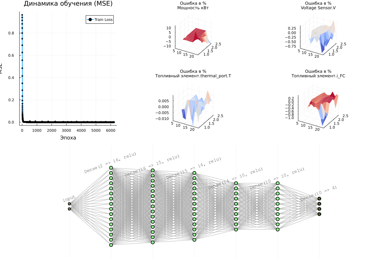
# Graph 1: Learning Curves
p_loss = plot(1:n_epochs, train_losses, label="Train Loss", lw=2, marker=:circle, markersize=2)
title!(p_loss, "Learning Dynamics (MSE)")
xlabel!(p_loss, "Era")
ylabel!(p_loss, "MSE")

println("Received Error value (MSE): ", best_loss)

# Surface graphs for all target variables
surface_plots = [plot_prediction_errors(model, X_train_norm, y_train_norm,
  X_train_mean, X_train_std, y_train_mean, y_train_std, i, adj_vars,
  title=out_vars[i])
  for i in 1:n_targets]

# Displaying all the graphs together
l = @layout [a{0.3w} b{0.7w}]
plot(plot(p_loss, plot(surface_plots...),layout=l), plot(model), layout=(2,1), size=(1200,900))

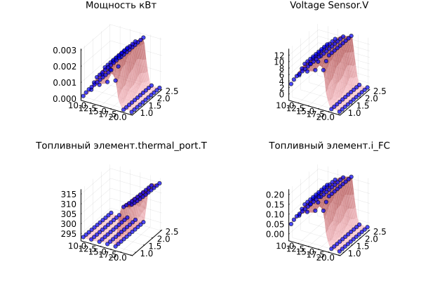
Полученное значение ошибки (MSE): 2.0551358e-6

Let's check how forecasts and initial data are combined.:

plot([plot_predictions(model, X_train_norm, y_train_norm, X_train_mean, X_train_std, y_train_mean, y_train_std, i, title=out_vars[i]) for i in 1:n_targets]...)

Notes on the learning process

Training is conducted several times, and the best model is selected. Each training run returns us a new neural network, and we need to remove the dependence on the initial parameters.
There is no division into a training and test subset. If there are many training points in the table, it is better to implement this separation and not risk overfitting.
The data for the neural network ** is normalized**. The training process uses data of very different scales (volts, kilometers, ...), and in order not to harm the quality of the forecast, the data is reduced to a single normal distribution.
It takes the most time to draw graphs. Otherwise, there is no need to worry about the learning rate, it is very high.
Any change in the parameters for the better is likely to improve the quality of approximation by the neural network, but increasing the capacity will bring retraining closer.

Conclusion

We have presented a methodology for creating a neural network based on the inputs and outputs of a physical model. Using it, you can package any model into a neural network and use it for forecasts.

Row	FuelCell/Давление водорода (бар)/Value	FuelCell/Подача топлива/slope
	Float64	Float64
1	2.0	0.833333
2	4.0	0.833333
3	6.0	0.833333
4	8.0	0.833333

Row	block	param	units	delta	lower	upper
	String	String15	String7	String15	String15	String15
1	FuelCell/Давление водорода (бар)	Value		2.0	2.0	20.0
2	FuelCell/Подача топлива	slope		10/60	50/60	150/60