Let's build a map of temperatures, precipitation, and weather events.
In this example, we want to show the possibilities of working with the map of Russia and weather services.
Let's start with the example after installing several libraries and configuring the environment.
]add Shapefile, GeoJSON
gr()
Uploading data using the OpenMeteo API
First of all, we will download the data for each point of the coordinate grid set by latitude and longitude.
Collecting weather data can take quite a long time. From the OpenMeteo open and free source, collecting terrain and weather data takes about 4 minutes for a map resolution of 4 degrees (with a 0.1 s delay between requests) and 7 minutes for a resolution of 2 degrees. This is acceptable for a training example, but for more serious work it is better to use a more productive API for commercial services.
# Uncomment it to download the latest data.
using Dates
target_date = Dates.Date(2026, 03, 08);
target_precision = 4;
target_hour = 12;

# include("get_meteo_data.jl")
# df_final = get_meteo_data( target_date, target_hour, target_precision );
# first( df_final, 5 )
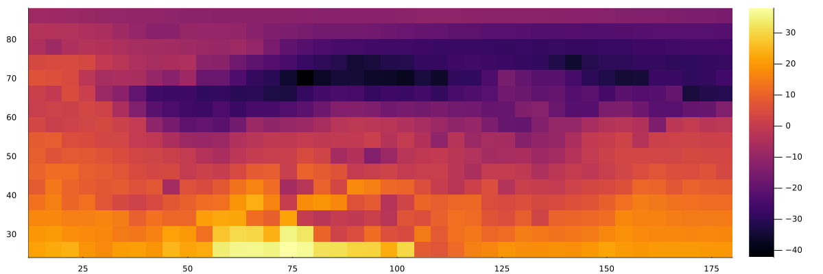
If you open the downloaded data and build a simple "heat map" using heatmap, we can construct the following image:
using CSV, DataFrames

df = CSV.read("The weather_russia is full.csv", DataFrame, types=[Int64, Int64, Float32, String, Float32, Float32, Float32, Float32], missingstring=["NA", "N/A", ""])
df = filter(r->!ismissing(r.temperature), df)
m = Matrix(permutedims(unstack(df, :longitude, :latitude, :temperature)[!, 2:end]))
heatmap(sort(unique(df.longitude)), sort(unique(df.latitude)), m, size=(1200,400))
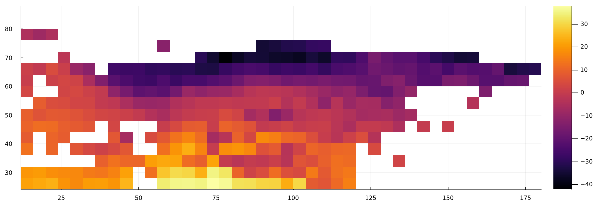
Filtering of land areas
Since we have also uploaded information about where each point of the matrix falls — on the water or not on the earth's surface, we can output such a graph:
m_temp = Matrix(permutedims(unstack(df, :longitude, :latitude, :temperature)[!, 2:end]))
m_land = Matrix(permutedims(unstack(df, :longitude, :latitude, :surface type)[!, 2:end]))
m_filtered = ifelse.(m_land .== "land", m_temp, NaN)
heatmap(sort(unique(df.longitude)), sort(unique(df.latitude)), m_filtered, size=(1200,400))
A small function for loading map borders from a file f It will allow us to plan the further course of work.:
# Function for uploading polygons from a GeoJSON file
load_borders(f) = [ [(p[1],p[2]) for p in poly] for f in JSON.parsefile(f)["features"] for geom in [f["geometry"]] for g in (geom["type"]=="MultiPolygon" ? geom["coordinates"] : [geom["coordinates"]]) for poly in g ];
Now you can put a map on top of the matrix.:
borders = load_borders("Russia_0.01.geojson")

lons = sort(unique(df.longitude)); lats = sort(unique(df.latitude));
# Creating a heatmap
p = heatmap(lons, lats, m_filtered[end:-1:1, :],
             yflip=true, size=(1200,400), xlims=(18,190), ylims=(35,85), xlabel="Longitude", ylabel="Width",
             color=:thermal, clims=(-40,30), colorbar_title="Temperature (°C)")
# Adding borders
for poly in borders
    xs = [point[1] for point in poly]; ys = [point[2] for point in poly]
    push!(xs, xs[1]); push!(ys, ys[1]) # Closing the polygon
    ys_flipped = [minimum(lats) + maximum(lats) - y .+ 9 for y in ys] # We take yflip into account
    plot!(p, xs .- 3, ys_flipped, linecolor=:red, linewidth=1.5, alpha=0.7, label="")
end

display(p)
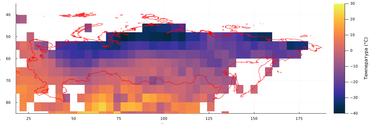
It turned out to be quite difficult to correlate the two graphs, besides, we see that many points on the coast did not fall into the discretization. But we plan to build such a schedule when we don't need very accurate accounting.
Let's compare the two functions of determining whether a point in the matrix belongs to the map shown in the file:
include("geo_poly_functions.jl")

lats = 36:target_precision:87
lons = 14:target_precision:200

crude_matrix = [point_in_russia(lon, lat, borders) for lat in lats, lon in lons]
smooth_matrix = [land_weight(lon, lat, borders, 1.0) for lat in lats, lon in lons]

plot(
    heatmap(lons, lats, crude_matrix[end:-1:1, :], yflip = true, aspect_ratio=1.5),
    heatmap(lons, lats, smooth_matrix[end:-1:1, :] .> 0.001, yflip = true, aspect_ratio=1.5),
    size=(1200,250)
)
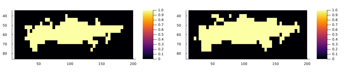
The map on the right will suit us much more, especially since by changing the threshold when building a mask for the map on the right, we can control the rendering of finer details and build exactly the map that best reflects the visual intent.
And now we can finally build a great weather event map.:
using CSV, DataFrames

# A function for converting the weather code of the WMO into emojis
function weathercode_to_emoji(code)
    if code == 0                 return "☀️"  # Clearly
    elseif code in [1, 2, 3]     return "☁️"  # Cloudy
    elseif code in [45, 48]      return "🌫️"  # Fog
    elseif code in [51, 53, 55]  return "🌧️"  # Drizzle
    elseif code in [56, 57]      return "🌨️"  # Icy drizzle
    elseif code in [61, 63, 65]  return "💧"  # Rain
    elseif code in [66, 67]      return "🌨️"  # Freezing rain
    elseif code in [71, 73, 75]  return "❄️"  # Snow
    elseif code == 77            return "🌨️"  # Snow groats
    elseif code in [80, 81, 82]  return "💧"  # Rainfall
    elseif code in [85, 86]      return "☃️"  # Snowfall
    elseif code == 95            return "⛈️"  # Thunderstorm
    elseif code in [96, 99]
        return "⛈️"  # Thunderstorm with hail
    else
        return "❓"
    end
end

# Uploading data
df = CSV.read("The weather_russia is full.csv", DataFrame, types=[Int64, Int64, Float32, String, Float32, Float32, Float32, Float32], missingstring=["NA", "N/A", ""])
df1 = filter(r->!ismissing(r.weather_code), df)
df1 = filter([:latitude, :longitude] => (lat,lon) -> land_weight(lon, lat, borders, 1.0) .> 0.001, df1)
lats, lons = sort(unique(df1.latitude)), sort(unique(df1.longitude))
emoji_matrix = fill("🟩", length(lats), length(lons))
emoji_dict = Dict((r.latitude, r.longitude) => weathercode_to_emoji(round(Int32, r.weather_code)) for r in eachrow(df1))
emoji_matrix = [get(emoji_dict, (lat, lon), "🟩") for lat in lats, lon in lons]

# We output the matrix line by line
for i in length(lats):-1:1
    println( join(emoji_matrix[i, :]) )
    println( join(emoji_matrix[i, :]) ) # Let's repeat each line twice.
end
println("Legend: it's clear |️ cloudy | 🌧️ rain | ❄️ snow | ☃️ let it Snow | ⛈️ thunderstorm | 🌫️ fog | ❓ no data")
Conclusion
We performed a small cartography exercise, uploaded a GeoJSON file and worked with scalar values from CSV tables, getting an interesting visualization as a result.