Approximation of a function by a polynomial
Introduction
In computational mathematics and experimental data processing, one of the key tasks is to restore analytical dependence on a discrete set of observations. Often, the true law describing a physical process is unknown or too complex for direct analysis, and the source data contains unavoidable measurement errors. In such cases, it becomes necessary to find a relatively simple function that best describes the available points in the sense of the minimum standard deviation. The classical least squares method solves this problem.
Importing libraries
In this example, we will need a library LinearAlgebra for operations with matrices and Printffor tabular output of results.
using LinearAlgebra, Printf
Function definition
Let's define the function under study. In this example, we are examining the sinc function (cardinal sine).
f(x) = x == 0 ? 1.0 : sin(x)/x
Table of function values
In order to select the polynomial that best describes the behavior of the function under study, it is first necessary to set specific values of this function at specific points. Let's define the step and interval, and build a table of function values.
a = 0
b = 16
step = 1.0

X = collect(a:step:b)
Y = [f(x) for x in X]

println("The table of the initial values of the function:\n")
for i in eachindex(X)
    @printf("X = %.4f, Y = %.6f\n", X[i], Y[i])
end
The least squares method
We implement the least squares method for selecting the coefficients of a polynomial of a given degree. To do this, it is necessary to solve a system of normal equations:
Where:
As a result, we obtain an array of coefficients of the desired polynomial, which best approximates the initial data (in the sense of the standard deviation).
MNC function(x, y, degree)
    M = [x[i]^j for i in 1:length(x), j in 0:degree]
    return (M' * M) \ (M' * y)
end
Definition of polynomials
In general, a polynomial of degree to approximate the function using the least squares method, it looks like this:
Let's define and compare polynomials of different degrees to approximate the function under study. As a result, we get a table of coefficients for the polynomials, which we will use in the future to calculate the values at new points and visually compare with the original function. This allows us to evaluate how increasing the degree of the polynomial affects the quality of the approximation.
degrees = [1, 3, 5, 7, 9]
N = Dict()

println("The coefficients of the polynomials of the best RMS approximation:")

for d in degrees
    K = MNC(X, Y, d)
    N[d] = K

    println("\nstep = $d")
    for i in 1:length(K)
        @printf("a%d = %.6f\n", i-1, К[i])
    end
end
Let's compare the original function with the obtained polynomials for a detailed analysis of the approximation quality. As a result, we will see how each polynomial approximates the original function over the entire interval.
w = 0.1
X = collect(a:w:b)

function Value(K, x)
    sum(K[i]* x^(i-1) for i in 1:length(K))
end

println("A table of function values and polynomials:")

for x in X
    @printf("\nx = %.4f | f(x)=%.6f", x, f(x))

    for d in degrees
        value = Value(N[d], x)
        @printf(" | P%d=%.6f", d, значение)
    end
end
Approximation by a 1st-order polynomial
Let's construct graphs for visual comparison of the function and its approximation by a first-order polynomial.
d = 1
график = plot(X, [f(x) for x in X], label="f(x)=sin(x)/x", lw=2)
plot!(X, [Значение(П[d], x) for x in X], label="The $d-th order polynomial",
xlabel="X", ylabel="Y", lw=2, legend=:right)
display(graph)
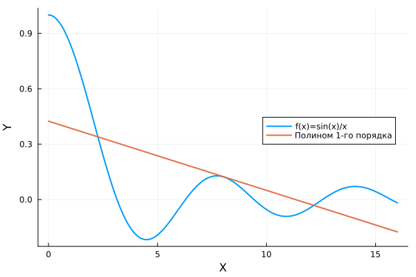
A first-order polynomial is a linear function. Obviously, there is no overlap with the function under study.
Approximation by a 3rd-order polynomial
Let's construct graphs for visual comparison of the function and its approximation by a third-order polynomial.
d = 3
график = plot(X, [f(x) for x in X], label="f(x)=sin(x)/x", lw=2)
plot!(X, [Значение(П[d], x) for x in X], label="The $d-th order polynomial",
xlabel="X", ylabel="Y", lw=2, legend=:right)
display(graph)
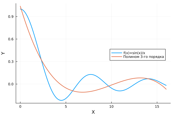
A 3rd-order polynomial is a cubic function, and the match is getting closer.
Approximation by a 5th order polynomial
Let's construct graphs for visual comparison of the function and its approximation by a fifth-order polynomial.
d = 5
график = plot(X, [f(x) for x in X], label="f(x)=sin(x)/x", lw=2)
plot!(X, [Значение(П[d], x) for x in X], label="The $d-th order polynomial",
xlabel="X", ylabel="Y", lw=2, legend=:right)
display(graph)
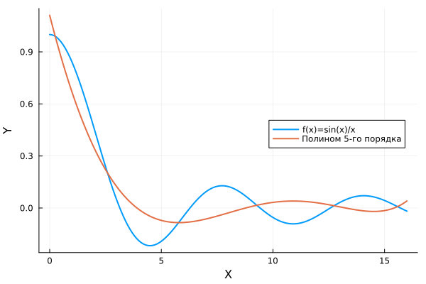
When approximated by a 5th order polynomial, the match gets even closer.
Approximation by a 7th-order polynomial
Let's build graphs for visual comparison of the function and its approximation by a seventh-order polynomial.
d = 7
график = plot(X, [f(x) for x in X], label="f(x)=sin(x)/x", lw=2)
plot!(X, [Значение(П[d], x) for x in X], label="The $d-th order polynomial",
xlabel="X", ylabel="Y", lw=2, legend=:right)
display(graph)
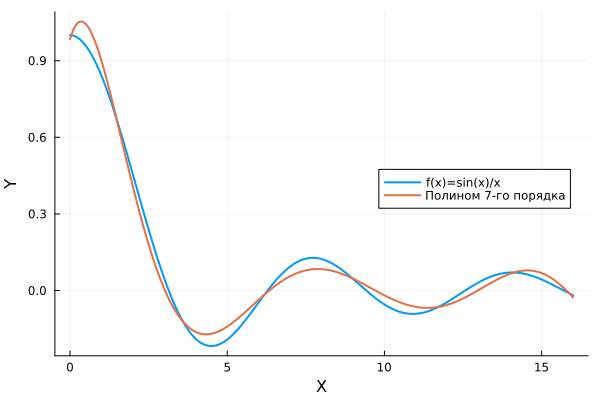
When approximated by a 7th-order polynomial, the match becomes even closer than when approximated by a 5th-order polynomial.
Approximation by a 9th-order polynomial
Let's build graphs for visual comparison of the function and its approximation by a ninth-order polynomial.
d = 9
график = plot(X, [f(x) for x in X], label="f(x)=sin(x)/x", lw=2)
plot!(X, [Значение(П[d], x) for x in X], label="The $d-th order polynomial",
xlabel="X", ylabel="Y", lw=2, legend=:right)
display(graph)
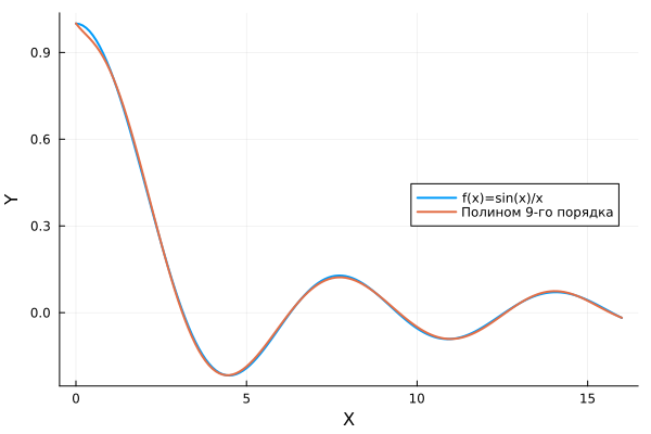
When approximated by a 9th-order polynomial, the function under study practically coincides with the polynomial. Thus, it can be concluded that the higher the order of the polynomial, the higher its coincidence with the function under study.
Conclusion
In this example, the classical least squares polynomial approximation problem was numerically implemented and investigated, which is a fundamental tool in a wide variety of fields of activity where it is necessary to restore dependencies on noisy or discrete data.:
-
Physics and engineering — processing of experimental results (for example, approximation of volt-ampere characteristics, calibration of sensors, smoothing of signals).
-
Economics and Finance — building time series trends, forecasting prices, and analyzing market indicators.
-
Biology and medicine — modeling of dose dependencies, population growth analysis, processing of clinical trial data.
-
Geophysics and astronomy — extraction of a useful signal against a background of noise, interpolation of satellite data.
-
Machine learning — data generalization (linear and polynomial regression) as the basis of many more complex algorithms.
Thus, the approach considered in the example is not limited to a purely educational task, but forms the basis for a variety of applied numerical methods. Choosing Engee allows you to further scale calculations to large amounts of data without loss of performance, which is especially important when solving real engineering and scientific problems.