Parametric analysis and dynamic visualization of the Lorentz attractor

Introduction

In this example, we study the influence of control parameters on the topology of the phase trajectories of the Lorentz system. Unlike static analysis with fixed parameter values, the dynamic visualization method is used here, which makes it possible to observe the evolution of the attractor structure in real time with continuous parameter changes.

The Lorentz system is described by the following system of nonlinear differential equations:

where — Prandtl's number, — the normalized Rayleigh number, is a geometric parameter that characterizes the ratio of the horizontal and vertical scales of a convective cell.

Let's do the research in two directions.:

Kinematic analysis — visualization of the attractor formation process by sequentially constructing a phase trajectory with simultaneous rotation of the observation point, which allows us to view the structure of the attractor from various angles.
Parametric analysis is the study of the transformation of a phase portrait when each of the control parameters is varied according to a harmonic law. The parameters change according to the following laws:

This approach makes it possible to identify bifurcation transitions and assess the sensitivity of the system to changes in each of the parameters individually, as well as when they are jointly adjusted.

Let's define the integration step , which will be used in all numerical experiments. The value is chosen based on the condition of ensuring the stability of the explicit Euler method and sufficient accuracy of reproducing the phase trajectory.

Δt = 0.01

Kinematic analysis: construction of an attractor in an evolutionary view

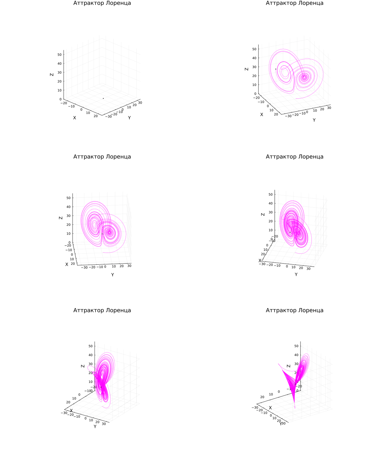
Let's create an animation demonstrating the evolution of the Lorentz system's phase trajectory over time. Unlike the static representation of the complete attractor, here the trajectory is displayed sequentially, point by point, which allows us to observe the dynamics of the formation of a strange attractor.

The system parameters are fixed in the classical chaotic configuration:

The initial conditions are chosen near the origin:

The integration is performed by the explicit first-order Euler method in steps on the interval conventional time units ($N = 10\text{⁴} $iterations). For animation, thinning is used in increments of 100 points, which corresponds to the display of each hundredth state of the system. The camera rotates slowly around the vertical axis according to the law:

where — the number of the displayed point.

σ = 10.0
β = 8.0/3.0
ρ = 28.0
dt = 0.01
N = 10000

x = zeros(N)
y = zeros(N)
z = zeros(N)
x[1] = 1.0
y[1] = 1.0
z[1] = 1.0

for i in 1:N-1
    dx = σ * (y[i] - x[i])
    dy = x[i] * (ρ - z[i]) - y[i]
    dz = x[i] * y[i] - β * z[i]
    x[i+1] = x[i] + dt*dx
    y[i+1] = y[i] + dt*dy
    z[i+1] = z[i] + dt*dz
end

w = 100
i = 1:w:N
anim = @animate for i in and
    plot3d(
        x[1:i], y[1:i], z[1:i],
        linecolor = :magenta,
        linewidth = 0.5,
        label = "",
        xlabel = "X", ylabel = "Y", zlabel = "Z",
        xlims = (-25, 25), ylims = (-35, 35), zlims = (0, 55),
        aspect_ratio = :equal,
        background_color = :white,
        camera = (45 + 0.01*i, 25), 
        # dpi = 100,
        size = (640, 480),
        title = "The Lorentz attractor",
        titlecolor = :black
    )
    
    scatter3d!(
        [x[i]], [y[i]], [z[i]],
        color = RGB(1.0, 0.3, 0.2),
        markersize = 1,
        label = ""
    )
end

gif(anim, "Lorenz_Attractor_1.gif", fps = 15)

Parametric analysis: the influence of control parameters on the structure of the attractor

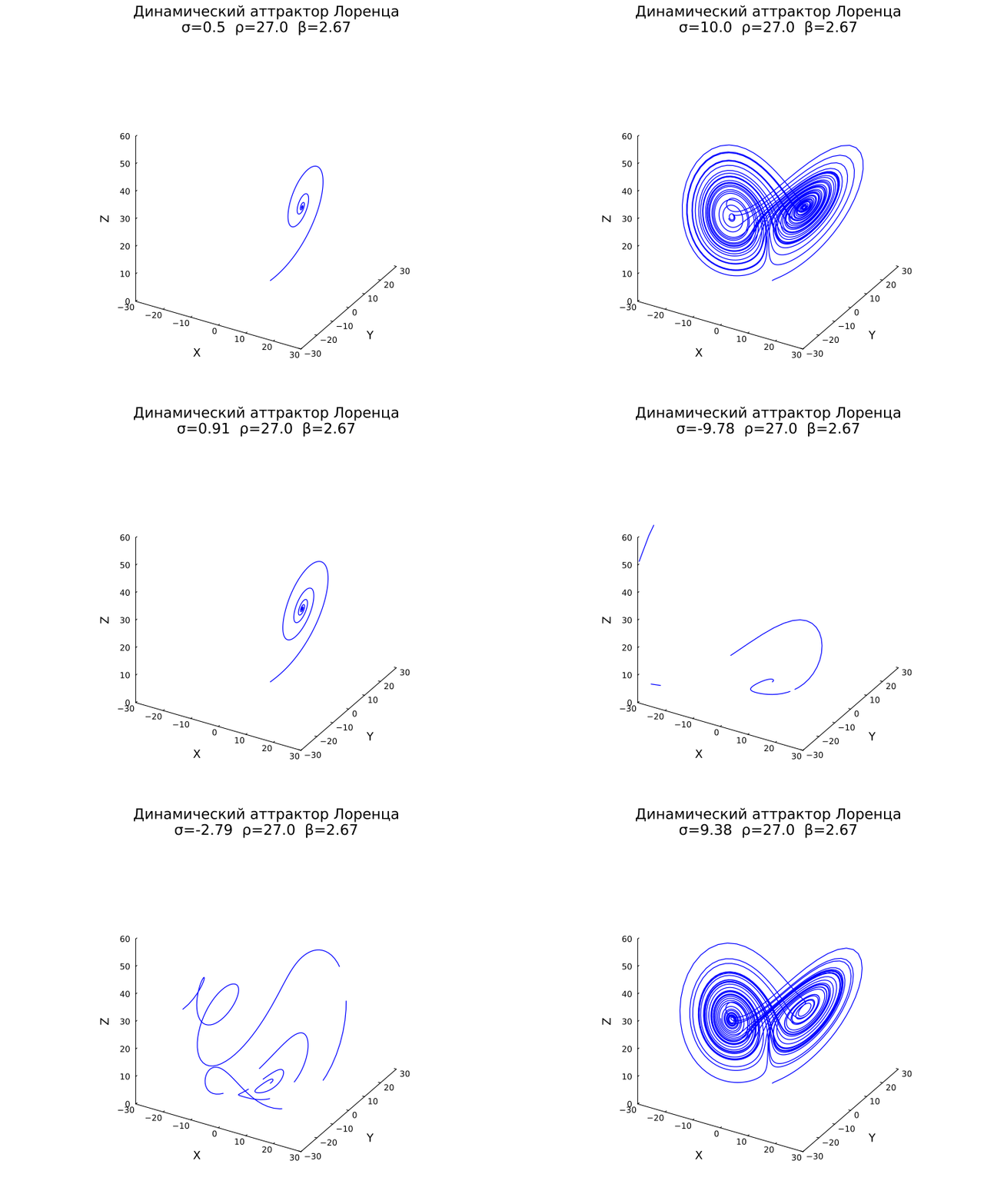
We study the system's response to a harmonic change in each of the three control parameters. For each animation, a separate numerical integration of the system is performed with fixed values of two parameters and a changing third. The number of iterations for each frame is

N = 4000

Dynamic parameter (Prandtl's number).

Parameter determines the relationship between the kinematic viscosity and the thermal conductivity of the medium. By The dissipative effects in the equation for the velocity of the fluid dominate over the thermal ones, which leads to the degeneration of chaotic dynamics. When zoomed in The system goes into a highly chaotic mode.

Setting the law of parameter change:

The other parameters are fixed:

frames = 1:150
σ_values = zeros(length(frames))
β_values = zeros(length(frames))
ρ_values = zeros(length(frames))

for (idx, f) in enumerate(frames)
    σ_values[idx] =  10*sin(f*0.05)
    β_values[idx] = 8/3
    ρ_values[idx] = 27
end

anim = @animate for (idx, f) in enumerate(frames)
    σ = σ_values[idx]
    β = β_values[idx]
    ρ = ρ_values[idx]
    x = zeros(N)
    y = zeros(N)
    z = zeros(N)
    x[1] = 1.0
    y[1] = 1.0
    z[1] = 1.0
    
    for n in 1:N-1
        dx = σ * (y[n] - x[n])
        dy = x[n] * (ρ - z[n]) - y[n]
        dz = x[n] * y[n] - β * z[n]
        x[n+1] = x[n] + Δt * dx
        y[n+1] = y[n] + Δt * dy
        z[n+1] = z[n] + Δt * dz
    end
    
    plot3d(
        x, y, z,
        linecolor = RGB(0, 0, 1),
        linewidth = 1.2,
        label = "",
        xlabel = "X", ylabel = "Y", zlabel = "Z",
        xlims = (-30, 30),
        ylims = (-30, 30),
        zlims = (0, 60),
        aspect_ratio = :equal,
        title = "Dynamic Lorentz attractor\nσ=$(round(σ, digits=2))  ρ=$(round(ρ, digits=2))  β=$(round(β, digits=2))",
        titlecolor = :black,
        background_color = :white,
        grid = false,
        legend = false, 
        size = (640, 480)
    )
end

gif(anim, "Lorenz_Attractor_2.gif", fps = 15)

Dynamic parameter (geometric parameter).

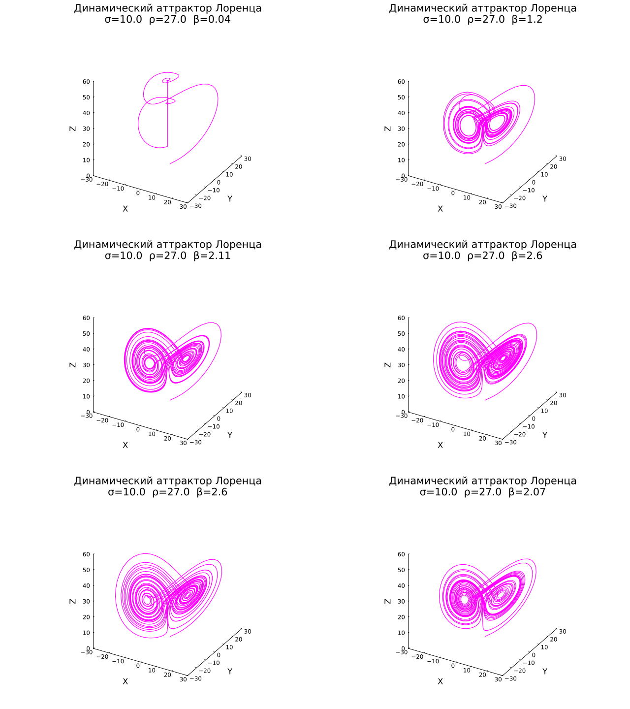
Parameter characterizes the ratio of the characteristic horizontal and vertical scales of a convective cell. Change it leads to a deformation of the phase portrait: at low values, the attractor is compressed along the axis at high temperatures, it stretches out, and the chaotic regime can collapse.

Setting the law of parameter change:

The other parameters are fixed:

frames = 1:150

σ_values = zeros(length(frames))
β_values = zeros(length(frames))
ρ_values = zeros(length(frames))

for (idx, f) in enumerate(frames)
    σ_values[idx] =  10
    β_values[idx] = 8/3*sin(f*0.015)
    ρ_values[idx] = 27
end

anim = @animate for (idx, f) in enumerate(frames)
    σ = σ_values[idx]
    β = β_values[idx]
    ρ = ρ_values[idx]
    
    x = zeros(N)
    y = zeros(N)
    z = zeros(N)
    x[1] = 1.0
    y[1] = 1.0
    z[1] = 1.0
    
    for n in 1:N-1
        dx = σ * (y[n] - x[n])
        dy = x[n] * (ρ - z[n]) - y[n]
        dz = x[n] * y[n] - β * z[n]
        x[n+1] = x[n] + Δt * dx
        y[n+1] = y[n] + Δt * dy
        z[n+1] = z[n] + Δt * dz
    end
    
    plot3d(
        x, y, z,
        linecolor = RGB(1, 0, 1),
        linewidth = 1.2,
        label = "",
        xlabel = "X", ylabel = "Y", zlabel = "Z",
        xlims = (-30, 30),
        ylims = (-30, 30),
        zlims = (0, 60),
        aspect_ratio = :equal,
        title = "Dynamic Lorentz attractor\nσ=$(round(σ, digits=2))  ρ=$(round(ρ, digits=2))  β=$(round(β, digits=2))",
        titlecolor = :black,
        background_color = :white,
        grid = false,
        legend = false, 
        size = (640, 480)
    )
end

gif(anim, "Lorenz_Attractor_3.gif", fps = 15)

Dynamic parameter (Rayleigh number).

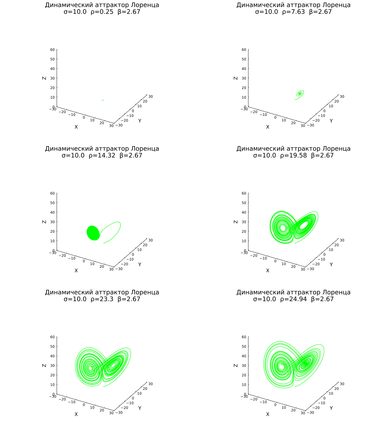
The parameter p characterizes the intensity of heating from below and is the main bifurcation parameter. By The system has a single stable singular point corresponding to the state of thermal conductivity without convection. With the growth A sequence of bifurcations occurs: the loss of stability of the stationary solution, the birth of a limit cycle, and, finally, the transition to a chaotic regime.

Setting the law of parameter change:

The other parameters are fixed:

frames = 1:150

σ_values = zeros(length(frames))
β_values = zeros(length(frames))
ρ_values = zeros(length(frames))

for (idx, f) in enumerate(frames)
    σ_values[idx] =  10
    β_values[idx] = 8/3
    ρ_values[idx] = 25*sin(f*0.01)
end

anim = @animate for (idx, f) in enumerate(frames)
    σ = σ_values[idx]
    β = β_values[idx]
    ρ = ρ_values[idx]
    
    x = zeros(N)
    y = zeros(N)
    z = zeros(N)
    x[1] = 1.0
    y[1] = 1.0
    z[1] = 1.0
    
    for n in 1:N-1
        dx = σ * (y[n] - x[n])
        dy = x[n] * (ρ - z[n]) - y[n]
        dz = x[n] * y[n] - β * z[n]
        x[n+1] = x[n] + Δt * dx
        y[n+1] = y[n] + Δt * dy
        z[n+1] = z[n] + Δt * dz
    end
    
    plot3d(
        x, y, z,
        linecolor = RGB(0, 1, 0),
        linewidth = 1.2,
        label = "",
        xlabel = "X", ylabel = "Y", zlabel = "Z",
        xlims = (-30, 30),
        ylims = (-30, 30),
        zlims = (0, 60),
        aspect_ratio = :equal,
        title = "Dynamic Lorentz attractor\nσ=$(round(σ, digits=2))  ρ=$(round(ρ, digits=2))  β=$(round(β, digits=2))",
        titlecolor = :black,
        background_color = :white,
        grid = false,
        legend = false,
        size = (640, 480)
    )
end

gif(anim, "Lorenz_Attractor_4.gif", fps = 15)

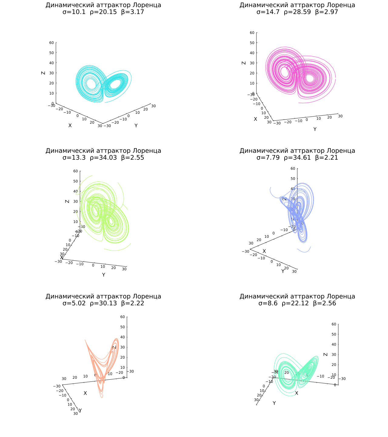
Joint variation of all control parameters

Consider the simultaneous harmonic variation of all three control parameters with different frequencies, amplitudes, and phases. This approach makes it possible to observe a complex interference of parametric effects and identify areas of parametric space in which the system demonstrates the most extensive dynamics.

Let's set the laws for changing the parameters:

Note that the parameter β is modulated according to the cosine law, which introduces a phase shift of π/2 relative to the sinusoidal modulations σ and p. The modulation frequencies also differ, which creates incommensurable wave periods and ensures dense filling of the studied area of the parametric space.

frames = 1:300

σ_values = zeros(length(frames))
β_values = zeros(length(frames))
ρ_values = zeros(length(frames))

colors = zeros(length(frames), 3)

for (idx, f) in enumerate(frames)
    σ_values[idx] = 10 + 5*sin(f*0.02)
    β_values[idx] = 8/3 + 0.5*cos(f*0.015)
    ρ_values[idx] = 20 + 15*sin(f*0.01)
    
    colors[idx, 1] = 0.2 + 0.8*abs(sin(f*0.02))
    colors[idx, 2] = 0.2 + 0.8*abs(sin(f*0.02 + 2π/3))
    colors[idx, 3] = 0.2 + 0.8*abs(sin(f*0.02 + 4π/3))
end

anim = @animate for (idx, f) in enumerate(frames)
    σ = σ_values[idx]
    β = β_values[idx]
    ρ = ρ_values[idx]
    
    x = zeros(N)
    y = zeros(N)
    z = zeros(N)
    x[1] = 1.0
    y[1] = 1.0
    z[1] = 1.0
    
    for n in 1:N-1
        dx = σ * (y[n] - x[n])
        dy = x[n] * (ρ - z[n]) - y[n]
        dz = x[n] * y[n] - β * z[n]
        x[n+1] = x[n] + Δt * dx
        y[n+1] = y[n] + Δt * dy
        z[n+1] = z[n] + Δt * dz
    end
    
    rgb_color = RGB(colors[idx, 1], colors[idx, 2], colors[idx, 3])
    
    plot3d(
        x, y, z,
        linecolor = rgb_color,
        linewidth = 1.2,
        label = "",
        xlabel = "X", ylabel = "Y", zlabel = "Z",
        xlims = (-30, 30),
        ylims = (-30, 30),
        zlims = (0, 60),
        aspect_ratio = :equal,
        title = "Dynamic Lorentz attractor\nσ=$(round(σ, digits=2))  ρ=$(round(ρ, digits=2))  β=$(round(β, digits=2))",
        titlecolor = :black,
        background_color = :white,
        grid = false,
        legend = false,
        camera = (45 + f*0.5, 25), 
        size = (640, 480)
    )
end

gif(anim, "Lorenz_Attractor_5.gif", fps = 15)

Conclusion

In this example, we performed a parametric study of the Lorentz system using dynamic visualization. Main results:

Kinematic analysis clearly demonstrated the process of forming a strange attractor and its fractal structure.
Parametric analysis revealed bifurcation transitions with harmonic variation of each of the control parameters and determined the ranges of existence of chaotic regimes.
The joint variation of the parameters showed a complex interference of effects in a multidimensional parametric space.

The engineering applications of the results obtained cover the following areas:

Heat engineering and power engineering — optimization of heat exchangers and cooling systems based on understanding convective instabilities and transition to turbulence.
Laser technology — equations equivalent to the Lorentz system describe the dynamics of single-mode lasers; parametric analysis is useful in the development of radiation sources with specified characteristics.
Cryptography and communication — the property of exponential sensitivity to parameters is used in the design of chaotic sequence generators for encryption and hidden data transmission systems.
Chemical engineering — chaotic mixing modes similar to those observed in the Lorentz system are used to intensify mass transfer in reactors.

The developed dynamic visualization toolkit can be used to analyze other nonlinear systems, and the resulting graphical representation of the behavior of a nonlinear system can be used for chaos management tasks in technical applications.