Synthetic Queuing Systems Generator
Introduction
In the problems of queuing theory, especially when optimizing the distribution of flows in M/M/1 type network structures, the quality of the source data plays a key role: matrices of bandwidth (capacities) of communication channels and matrices of the intensity of external application flows. To verify, test, and compare the effectiveness of nonlinear optimization algorithms such as gradient methods or interior point methods, it is necessary to generate representative sets of test scenarios with controlled parameters of topology, sparsity, asymmetry, and system load.
In this example, a parameterized generator of synthetic queuing systems (CFOs) is implemented. Unlike the manual generation of the initial matrices, the generator allows you to automatically create multiple CFR configurations, varying the number of nodes, the degree of connectivity of the graph, statistical distributions of channel capacities and flow rates. The data obtained is exported in a standardized .xlsx format, which ensures direct compatibility with subsequent analysis stages, including optimization based on the M/M/1 model.
Thus, the result of executing this script is not only visualized CFR topologies, but also controlled test datasets. These kits are designed, in particular, for quantitative testing of the quality, convergence and performance of algorithms for optimizing queuing systems, allowing them to assess their stability with varying degrees of sparsity, channel asymmetry and competitive load levels.
CFR structure
The structure of the queuing system can be represented as a square matrix of the network size :
Where – the number of nodes in the network, – the total bandwidth of communication channels (graph branches) connecting nodes and directed from the node with the number to the node with the number .
The flow direction in queuing systems can also be represented as a square matrix of the size :
Where – the number of nodes in the network, – the amount of flow directed from the node with the number to the node with the number .
As a rule, in real systems there are no loop flows (flows from a node addressed to itself), respectively, the diagonals of the matrices are zero. However, for additional experiments, in this example it is possible to generate matrices with non-zero diagonals.
Attaching files and libraries
We will attach the necessary libraries. In this example, we will need libraries.:
LinearAlgebra– for matrix operations;XLSX,Printf– for data output and saving;Graphs, Colors, GraphPlot, SimpleWeightedGraphs– for displaying CFR in the form of graphs.
# EngeePkg.purge()
# import Pkg
# Pkg.add(["XLSX", "Graphs", "Colors", "Printf", "GraphPlot", "LinearAlgebra", "SimpleWeightedGraphs"])
using XLSX, Graphs, Colors, Printf, GraphPlot, LinearAlgebra, SimpleWeightedGraphs
We will also attach the necessary files with functions.:
flGplot.jl, flowGraph.jl, "netGraph.jl", nGplot.jl, sGplot.jl", simpGraph.jl – for displaying CFR in the form of graphs;
optiwrite.jl, "readqs.jl", qsdata.jl– for data output and saving.
foreach(include, ("flGplot.jl", "flowGraph.jl", "netGraph.jl", "nGplot.jl", "optiwrite.jl", "readqs.jl", "sGplot.jl", "simpGraph.jl","qsdata.jl"))
Initial parameters
Let's define the initial data.
Parameters of adjacency matrices:
- Number of nodes
- The degree of sparsity of the matrices (a parameter that sets the number of iterations of random zeroing of connections between nodes, which regulates the density of the network topology)
- Condition: is the diagonal zero (are there loops)
- Condition: is the matrix symmetric (for each outgoing communication line there is an incoming one);
Parameters of communication line capacities:
- Is the capacity matrix symmetrical (are the capacities of outgoing and incoming communication lines equal to each node)
- Conditions: are the capacities the same (are all capacities of communication lines equal, if equal, they are equal to the value of the minimum capacity)
- Minimum capacity
- Maximum capacity;
Flow Parameters:
- Condition: are there loop flows
- Condition: are the flows the same (are the intensities of all flows equal, if equal, then they are equal to the value of the minimum flow)
- Minimum flow
- Maximum flow
- The degree of sparsity of the flow matrices;
# Parameters of adjacency matrices
узлов = 9  # Number of nodes
разр = 2  # Degree of sparsity
диаг = true  # Is the diagonal zero
симм = false  # Is the matrix symmetric

# Parameters of communication line capacities
симм_ёмк = false  # Is the capacity matrix symmetrical
равно_ёмк = false  # Are the capacities the same
мин_ёмк = 1.0     # Minimum capacity
макс_ёмк = 12.0     # Maximum capacity
диаг_поток = false # Loop flows

# Flow Parameters
равно_поток = false # Are the flow rates the same
мин_поток = 1.5  # Minimum flow
макс_поток = 5.5  # Maximum flow
разр_поток = 4   # The degree of sparsity of the flow matrices
Matrix generation function
Let's define a function that accepts the initial data, and depending on them returns a matrix of capacities and adjacency of communication lines, as well as a matrix of directions and intensities of flows.
function RandQ(qN, spL, dZ, sM, syBw, smBw, minBw, maxBw, dZf, smFl, minFl, maxFl, spFl)

# Creating a matrix of ones and zeros
rM = ones(qN, qN)
for n = 1:spL
    rM = rM .* rand(0:1, qN, qN)
end

# Zeros on the diagonal
if dZ
    for m in 1:qN
        rM[m, m] = 0
    end
end

# Symmetry of the adjacency matrix
    if sM
        for p in 1:qN
            for q in p:qN
                rM[q, p] = rM[p, q]
            end
        end
    end

# Capacities of communication lines
if smBw
    nM = minBw .* rM
else
    nM = (minBw .+ (maxBw .- minBw) .* rand(qN)) .* rM
end

# Symmetry of the adjacency matrix
if syBw
    for p in 1:qN
        for q in p:qN
            nM[q, p] = nM[p, q]
        end
    end
end

# The matrix of flow directions
if smFl
    flM = minFl .* rand(0:1, qN, qN)
else
    flM = minFl .+ (maxFl .- minFl) .* rand(qN, qN)
end

# Sparsity of the flow direction matrix
for n in 1:spFl
        flM = flM .* rand(0:1, qN, qN)
end

# The zero diagonal of the flow direction matrix
if dZf
    for m in 1:qN
        flM[m, m] = 0
    end
end

return nM, flM
end
Creating and saving matrices
Referring to the matrix generation function, we will create several pairs of matrices (adjacencies and flows), depending on the specified number. Saving the created matrices to xlsx files:
-
NetMatrix.xlsx– matrices of capacities and adjacency of communication lines; -
FlowMatrix.xlsx– matrices of the intensities and directions of the flows.Each new matrix is created in a new sheet of each xlsx file. The number of sheets in each file corresponds to the number of pairs of matrices.
количество = 3   # The number of matrix pairs to create
QS = zeros(Float64, nodes, nodes, number)
Flows = zeros(Float64, nodes, nodes, number)
for q in 1:quantity
    nM, flM = RandQ(nodes, size, diag, simm, simm_emk, equil_emk, min_emk, max_emk, diag_flow, equil_flow, min_flow, max_flow, raz_flow)
    QS[:,:,q] = nM
    Flows[:,:,q] = flM
end
optiwrite(QS, "NetMatrix.xlsx", "Net")
optiwrite(Flows, "FlowMatrix.xlsx", "Flow")
Visualization
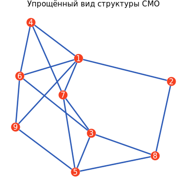
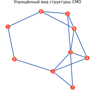
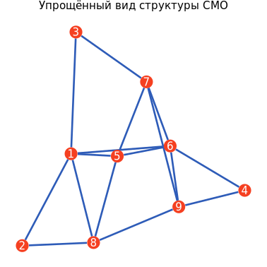
We will display the CFR parameters, as well as display them in the form of graphs.:
- simplified view of structures;
- full view of the structures indicating the directions and capacities of the communication lines;
- Intensity and direction of flows.
n = 1 # The number of the matrix pair
CFR, Streams = qsdata(n)
and, n = simpGraph(CFR);
Graph = sGplot(i, n)
display(Graph)
s, t, bW = netGraph(CFR);
ГрафСМО = nGplot(s, t, bW, "The structure of the queuing system");
display(GRAPHSMO)
nfl, nl, flG, flI = flowGraph(Streams);
ГрафПотоков = flGplot(flG, flI, nl, "Flow directions");
display(Graph streams)
.png)
.png)
n = 2 # The number of the matrix pair
CFR, Streams = qsdata(n)
and, n = simpGraph(CFR);
Graph = sGplot(i, n)
display(Graph)
s, t, bW = netGraph(CFR);
ГрафСМО = nGplot(s, t, bW, "The structure of the queuing system");
display(GRAPHSMO)
nfl, nl, flG, flI = flowGraph(Streams);
ГрафПотоков = flGplot(flG, flI, nl, "Flow directions");
display(Graph streams)
.png)
.png)
n = 3 # The number of the matrix pair
CFR, Streams = qsdata(n)
and, n = simpGraph(CFR);
Graph = sGplot(i, n)
display(Graph)
s, t, bW = netGraph(CFR);
ГрафСМО = nGplot(s, t, bW, "The structure of the queuing system");
display(GRAPHSMO)
nfl, nl, flG, flI = flowGraph(Streams);
ГрафПотоков = flGplot(flG, flI, nl, "Flow directions");
display(Graph streams)
.png)
.png)
Thus, by setting your own initial parameters, you can create your own pairs of matrices in a convenient xlsx format, visualize their structure as graphs and use them for further research.
Conclusion
The Queuing System Generator provides researchers and engineers with a tool for quickly creating synthetic but statistically plausible CFR configurations with a wide range of topological and load characteristics. The ability to generate multiple matrix pairs (capacities — flows) in a standardized format ensures reproducibility of experiments and serves as a basis for comparative analysis of various optimization algorithms.
In addition to the task of testing the performance and quality of optimization algorithms, the presented generator can be applied in practice in the following areas:
-
Telecommunication network design — to generate multiple load scenarios when choosing a topology and reserving channels.
-
Logistics and Supply chain management — for modeling alternative delivery routes with different capacity of logistics hubs.
-
Educational process — to create individual tasks on queuing theory and optimization methods.
-
Verification of analytical models — by comparing optimization results on synthetic data with known analytical solutions for special cases.
-
Load testing of software implementations of optimization algorithms — to assess their stability when increasing the problem dimension (number of nodes and threads) and the degree of sparsity of the graph.
Thus, the algorithm presented in this example is not only an auxiliary tool for data preparation, but also an independent tool for the systematic study of the properties of queuing systems and the behavior of numerical optimizers in conditions of varying structural complexity.