Diffraction of a Gaussian beam on an absorbing half-plane

In this problem, the propagation of a two-dimensional wave field near the boundary of an ideally absorbing half-plane is considered. The source is a Gaussian beam incident perpendicular to the edge of the screen. The main goal is to show how the wave "flows" into the area of the geometric shadow, forming a smooth field devoid of interference oscillations on the surface, which is typical for the Fock model. We will numerically solve the corresponding equation of the evolutionary type and visualize the amplitude of the field along the interface of the media.

The parabolic Leontovich—Fock equation

The Leontovich-Fock parabolic equation was solved by Vladimir Alexandrovich Fock together with Mikhail Alexandrovich Leontovich during the study of the propagation of radio waves around the curved surface of the Earth.

The difficulty of the task was that classical methods simply did not work in the so—called "Foca region" - the transition zone at the boundary of light and shadow. Imagine the surface of the Earth illuminated by a radio transmitter. Where the rays reach in a straight line (line of sight), everything is more or less clear. But further away, beyond the horizon, there is a shadow zone, where, as we know in practice, radio waves still penetrate. It was extremely difficult to describe this process mathematically.

This equation is obtained from the Helmholtz equation by isolating a rapidly oscillating multiplier propagating along the selected direction and neglecting the second derivative along the longitudinal coordinate. It describes the slow complex amplitude of the wave u(x,z) near the shadow boundary.

The equation is written as follows:

Here — coordinate along the direction of propagation, — transverse coordinate, — the wave number, and — the relative permittivity of the medium (depends only on ).

This equation tells us that the slow amplitude of the wave u varies along x in proportion to the curvature of its profile along z. Physically, this describes how a narrow beam spreads out and seeps into the shadow area as it spreads. For a computer, the derivatives need to be replaced with discrete analogues, so we cover the plane a grid with steps and , and the second derivative by we write through the values at three adjacent points: .

Knowing the field at some x, we want to find it in the next step. . The simple explicit method is unstable here, so we use the Crank—Nicholson scheme, which averages the second derivative between the current and the next layer.: , where — the matrix of the discrete second derivative. Having suffered the unknown to the left, and the known to the right, we get a system of linear equations with a tridiagonal matrix . By solving it at each step, we move the wave forward along the . To simulate the edge of the absorbing screen, after each step we forcibly adjust the amplitude in the node of the grid that corresponds to for everyone . This creates a visual diffraction pattern: the beam widens, and the part of it touching the boundary is irrevocably absorbed.

Decision

Let's consider a model problem for free space () with the boundary condition of ideal absorption on the half-plane: by . Initial field distribution at We define it as a Gaussian beam offset from the boundary. The evolution of software We will perform using a completely implicit finite difference scheme (the Crank—Nicholson method), which has good stability.

using LinearAlgebra

# --- Task parameters ---
k = 20.0          # The wave number
Lz = 10.0         # the size of the area in z
Nz = 300          # the number of nodes in z
dz = Lz / Nz
z = range(-Lz/2, Lz/2, length=Nz+1)[1:Nz]

Lx = 5.0
Nx = 200
dx = Lx / Nx
x_range = range(0, Lx, length=Nx+1)

# The initial Gaussian beam
z0 = 2.0
w0 = 0.5
u0 = @. exp(-((z - z0)/w0)^2)

# --- Discretization ---
main_diag = -2.0 * ones(Nz)
off_diag  = ones(Nz-1)
D2 = (1/dz^2) * (diagm(-1 => off_diag, 0 => main_diag, 1 => off_diag))
D2[1, end] = 1/dz^2
D2[end, 1] = 1/dz^2

alpha = -1im / (2k)
I_mat = Matrix{ComplexF64}(I, Nz, Nz)
A = I_mat - (alpha * dx/2) * D2
B = I_mat + (alpha * dx/2) * D2

zero_idx = argmin(abs.(z .- 0.0))

# --- March on x ---
u = copy(u0)
field_amplitude = zeros(Float64, Nz, Nx+1)
field_amplitude[:, 1] = abs.(u)

for n in 1:Nx
    u = A \ (B * u)
    u[zero_idx] = 0.0
    field_amplitude[:, n+1] = abs.(u)
end

# --- 3D surface ---
plot(
    x_range, z, field_amplitude,
    st = :surface,          # graph type — surface
    xlabel = "x (longitudinal coordinate)",
    ylabel = "z (transverse coordinate)",
    zlabel = "|u|",
    title = "Diffraction of a Gaussian beam at an absorbing half—plane (Leontovich-Fock equation)",
    camera = (45, 30),      # convenient viewing angle
    colorbar_title = "The amplitude",
    alpha = 0.9,            # slight transparency for better depth perception
    fillalpha = 0.8,
    linewidth = 0.1,        # a thin grid to avoid overloading the image.
    titlefont=font(10), guidefont=font(6)
)

# Let's add the edge line of the half-plane for clarity
plot!(
    [0, Lx], [0, 0], [0, 0],
    lw = 3, color = :black, linestyle = :dash, label = "Edge of the half-plane (z=0)"
)

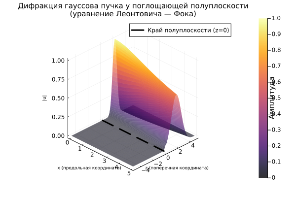
The graph shows how the Gaussian beam shifts and widens due to diffraction, and its amplitude near z = 0 tends to zero as it propagates beyond the edge of the half-plane.

Conclusion

The Leontovich—Fock parabolic equation makes it possible to efficiently calculate diffraction effects near the shadow boundary without having to solve the full wave equation. The demonstrated numerical solution by the Crank—Nicholson method is stable and easily scaled to more complex permittivity profiles, which makes it a convenient tool for analyzing the propagation of radio waves near the Earth's surface and in quasi-optics problems.