Multi-channel broadband direction finding system for small objects
The example considers the modeling of a multi-channel radar system for solving the problem of direction finding multiple targets. The target small objects are unmanned aerial vehicles (UAVs) - "quadcopter".
Before executing the script, it is recommended to clear the workspace using the command engee.clear(). If this is not required, you can delete or comment on this command. You can also choose the type of graph visualization: interactive or static. The control is implemented using a variable is_dinamic_plot.
engee.clear() # clearing the workspace
is_dinamic_plot = true # choosing the graph type:true (plotlyjs()) - interactive, false (gr()) - static
is_dinamic_plot ? plotlyjs() : gr()
Connecting auxiliary files and libraries
To implement the system in question, it is necessary to connect third-party libraries and auxiliary functions.:
let
    installed_packages = collect(x.name for (_, x) in Pkg.dependencies() if x.is_direct_dep)
    list_packages = ["JLD2","Hungarian"]
    for pack in list_packages
        pack in installed_packages || Pkg.add(pack)
    end
end

using LinearAlgebra,Hungarian,DataFrames
import JLD2

include("$(@__DIR__)/utils/plot_sig_and_spec.jl") # the function of building an oscillogram and a spectrogram
include("$(@__DIR__)/utils/viz_scene.jl") # the function of building a radar operation scenario
include("$(@__DIR__)/utils/calc_plot_rcs.jl") # backscatter diagram construction function
include("$(@__DIR__)/utils/sort_ang_mse.jl") # the function of sorting bearing estimates
include("$(@__DIR__)/utils/plot_spec_azel.jl") # the function of constructing a spatial spectrum
include("$(@__DIR__)/utils/calc_table_ang_analysis.jl") # table calculation function for accuracy analysis
1. Development of a system model of the radar operation scenario
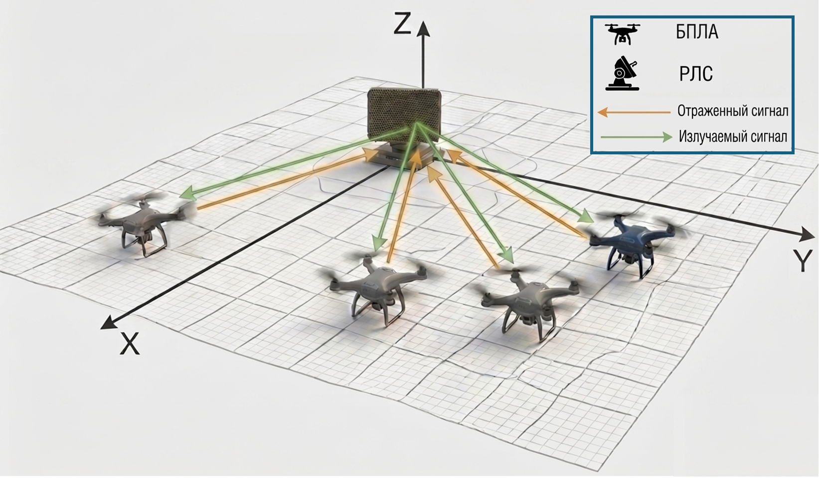
Let's consider the scenario of a multi-channel broadband direction finding system with multiple targets.
- It is assumed that the radar is located at the origin, oriented along the x axis. To solve the problem of determining the bearing, a rectangular phased array antenna (FAR) and a digital processing algorithm (MUSIC, MVDR, BeamScan) are used
- Four small-sized UAV objects of the "Quadcopter" type are moving towards the radar station against the x axis. Each of the objects has its own trajectory. The range to the targets is 1000-1500 meters, the speed is 130-150 m/s. The azimuthal directions to the target are within [-20, 20] degrees, the angular ones are [0, 30] degrees.
An approximate look of the scenario is shown in the figure below.
1.1 Description of the radar structure
Let us describe in more detail the structural scheme of the radar system model.:
-
ZS generator: A pulse signal with linear frequency modulation (LFM) is used as a probing signal;
-
Transmitter: The signal is amplified in the transmitter, taking into account the loss in the transmission path;
-
Transmitting headlight: A directional pattern (DN) is formed using a rectangular headlight;
-
Propagation medium: takes into account propagation attenuation, frequency dispersion, and weather effects;
-
Target: describes the DOR, taking into account the broadband spectrum of the signal and the trajectory of the target;
-
Transmitting headlight: the bottom is formed using a receiving broadband rectangular headlight,;
-
Receiver: implements the amplification of the received signal with the addition of its own thermal noise (LNA model).
-
Bearing algorithm: is one of the digital algorithms (MUSIC,BeamScan,MVDR) that determines the direction of the target in the azimuthal and angular planes;
The model's operation scheme is shown in the figure below.

1.2 Radar parameters
The key radar parameter is the carrier frequency value. When choosing the frequency range, it is necessary to take into account the tasks of radar, since the higher the value of the carrier frequency, the higher the attenuation and attenuation during propagation, while increasing the sensitivity to small objects.
When solving the problem of direction finding of small objects, it is advisable to use ranges commensurate with the size of targets (20-30 cm): L- or S-ranges. Let's choose the L-band (1-2 GHz) of the radar system, and take the carrier frequency value to be 1 GHz (λ ≈ 0.3 m).
# Fundamental radar parameters
fc = 1e9 # [Hz], carrier frequency
c = physconst("LightSpeed") # [m/s], the propagation speed of the signal
lambda = c / fc; # wavelength, m

println("Carrier frequency: $(FC*1E-9)GHz")
println("Speed of light: $c m/s")
println("Wavelength: $lambda m")
1.3 Parameters of the probed signal
As a probing pulse, we will select a signal with intra-pulse modulation - pulse LFM signal, with a stripe bw - 100 MHz, duration T - 10 microseconds and a borehole Q - 2. Such a signal is broadband because the ratio of the signal band to the carrier frequency is greater than 5% (in the example, 10%). The signal generation is implemented using a system object EngeePhased.LinearFMWaveform . Using the parameter n_pulses , n_groups_imps you can set the number of accumulation pulses per pack and the number of packs accordingly.
It is important that the broadband system requires setting the number of frequency sub-bands. NBand, within which the signal will be considered narrowband. The total bandwidth is determined by the sampling rate The width of the subrange is calculated as (1)
then the central frequencies of the sub-bands are calculated using the formula (2)
# --- Signal parameters ---
bw = 100e6; # LFM band, Hz
T = 10e-6; # Pulse duration, s
Q = 2 # pulse continuity
prf = round(1 / (Q * T);sigdigits = 15); # Pulse repetition rate (rounding if necessary)
type_dir = "Up" # frequency change direction ["Up","Down"]
type_sweep = "Positive"  # frequency change type ["Positive","Symmetrical"]
n_pulses = 2 # number of accumulation pulses
n_groups_imps = 2 # number of pulse bursts

fs = 2*bw; # Sampling rate, Hz
NBand = 64; # number of frequency sub-bands

T_coh = n_pulses/prf # the time of the coregent accumulation
ΔR = c/(2*bw) # range resolution, m
ΔV = lambda/(2*T_coh) # speed resolution, m/s
Rmin = c*T/2 # minimum one-digit range, m
Rmax = c/(2*prf) # maximum one-digit range, m
Vmax = lambda*prf/4 # maximum single-digit speed, m/s

# formation of the system object of the LFM signal generator
waveform = EngeePhased.LinearFMWaveform(
    SampleRate = fs, # Sampling rate, Hz
    PulseWidth = T, # Pulse duration
    PRF = prf, # Pulse repetition rate
    SweepBandwidth = bw,  # The LCHM band
    SweepDirection = "Up", # direction of frequency change
    SweepInterval = "Positive", # saw type, non-symmetrical or symmetrical
    OutputFormat = "Pulses", # output format type []
    NumPulses = n_pulses # number of pulses
);
We visualize the waveform and the spectrogram of the signal for a given number of pulses in 1 packet.
# calculation of the LFM signal
sig_lfm = waveform();

# construction of an oscillogram and a spectrogram
plot_sig_and_spec(sig_lfm;fs=fs,name_sig = "LCHM")
The tactical and technical characteristics of the formed vehicle are given below:
println("Sampling rate: $(round(fs*1e-6;sigdigits=5)) MHz")
println("Pulse duration: $(round(T*1e6;sigdigits=5)) microseconds")
println("Follow-up period: $(round(1e6/prf;sigdigits=5)) mks")
println("Repetition rate: $(round(prf*1e-3;sigdigits=5)) kHz")
println("Borehole: $(round(Q;sigdigits=5))")
println("Coherent accumulation time: $(round(T_coh*1e3;sigdigits=5)) ms")
println("Number of pulses per packet: $n_pulses")
println("Number of packs: $n_groups_imps")
println("Range resolution : $(round(ΔR;sigdigits=3)) m")
println("Speed resolution : $(round(ΔV;sigdigits=3)) m/s")
println("Maximum one-digit range : $(round(Rmax;sigdigits=3)) m")
println("Minimum one-digit range : $(round(Rmin;sigdigits=3)) m")
println("Maximum single-digit speed: $(round(Vmax;sigdigits=3)) m/s")
1.4 Antenna formation
A two-dimensional antenna array is required for direction finding in two directions - azimuth and elevation. The example uses the most common type, a rectangular equidistant headlight, which is set using the EngeePhased.URA. An isotropic radiator acts as an element of the headlights. - EngeePhased.IsotropicAntennaElement.
# antenna parameters
d = lambda /2 # the distance between the elements
freq_range = [fc-bw fc+bw] # frequency range of radiation
Nx = 24 # Number of elements on the X-axis (azimuth resolution)
Ny = 24 # Number of elements on the Y-axis (resolution by angle of location)
Δaz = rad2deg(lambda/(d*(Nx-1))) # azimuth resolution, deg
Δel = rad2deg(lambda/(d*(Ny-1))) # seat angle resolution, deg
# Total number of elements N = Nx * Ny

# WITH an isotropic antenna element
ant_elem = EngeePhased.IsotropicAntennaElement(
    FrequencyRange = freq_range, # frequency range
    BackBaffled = true # removing the backscatter of the antenna bottom
)

# creating a rectangular headlight
array = EngeePhased.URA(
    Element = ant_elem, # antenna element
    Size = [Nx Ny], # grid size
    ElementSpacing = [d d], # the distance between the elements
);
Visualize the directional pattern of the headlights using the function pattern.
# pattern(array,fc)
The parameters and characteristics of the rectangular headlamps are given below:
println("Distance between elements : $(round(d;sigdigits=3)) m")
println("Rectangular HEADLIGHT Dimensions: $(Nx)x$Ny [Nx, Ny]")
println("Frequency range of radiation: $(freq_range*1e-9) GHz")
println("Azimuth resolution: $(round(Δaz;sigdigits=3)) °")
println("Location angle resolution: $(round(Δel;sigdigits=3)) °")
1.5 Transmitting and receiving path
The next component of the radar is the ** receiving and transmitting path**. It performs 2 main tasks:
- Radiation of a probing signal into space in the form of an electromagnetic wave (EMW);
- Receiving the reflected signal from the target.
The transmission path includes 2 components: transmitter, which implements pre-amplification and headlights. The receiving path is similarly formed, including a receiving headlight and a preamp.
# Parameters of the receiving and transmitting path
Pt = 1e3 # W, peak power
Gtx = 20 # dB, gain of the transmitting antenna
LFtx = 1.5 # dB, losses in the transmission path

Grx = 20 # dB, gain of the receiving antenna
NF = 2 # dB, the noise coefficient of the receiving path
LFrx = 1.5 # dB, losses in the receiving path
TN = 290 # noise temperature
NP = physconst("boltzmann") * bw * TN; # W, noise power

# Creatures with a transmitter
transmitter = EngeePhased.Transmitter(
    Gain = Gtx, # transmitter gain
    PeakPower = Pt, # Peak power
    LossFactor=LFtx # losses in the transmission path
)

# Devices WITH broadband transmission lights
radiator = EngeePhased.WidebandRadiator(
    Sensor = array, # The bottom of the antenna element
    SampleRate = fs, # sampling rate
    CarrierFrequency = fc, # carrier frequency
    NumSubbands = NBand # number of frequency sub-bands
)

# devices WITH broadband receiving headlights
collector = EngeePhased.WidebandCollector(
    Sensor = array, # The bottom of the antenna element
    SampleRate = fs, # sampling rate
    CarrierFrequency = fc, # central frequency
    NumSubbands = NBand # number of frequency sub-bands
)

# creation of a receiving preamplifier (LNA)
receiver = EngeePhased.ReceiverPreamp(
    NoiseMethod="Noise power", # noise setting method ["Noise power", "Noise temperature"]
    Gain = Grx, # receiver gain, dB
    NoisePower = NP, # noise power
    LossFactor=LFrx, # losses in the receiving tract
    NoiseFigure = NF, # the noise factor in the path
    SampleRate = fs # sampling rate
);
The parameters and characteristics of the transceiver path are given below:
println("----------------- The transmitter-----------------------------")
println("Transmitter power: $(round(Pt*1e-3;sigdigits=5)) kW")
println("Transmitter gain: $(round(Gtx;sigdigits=5)) dB")
println("Transmission path loss: $(round(LFtx;sigdigits=5)) dB")
println("--------------------------------------------------------")
println("-----------------The receiver-----------------------------")
println("Receiver gain: $(round(Gtx;sigdigits=5)) dB")
println("Losses in the receiving path: $(round(LFtx;sigdigits=5)) dB")
println("Noise temperature: $(round(LFrx;sigdigits=5)) dB")
println("Noise level: $(round(NF;sigdigits=5)) dB")
println("Noise temperature: $(round(TN;sigdigits=5)) °C")
println("Noise power: $(round(NP;sigdigits=5)) W")
1.6 Digital processing unit (direction finder)
The last block of the radar is the direction finding algorithm. Such a block solves the problem of determining the direction of arrival of the signal and, as a result, the direction of the target object in relation to the radar. Consider the most used ones: "BeamScan", "MVDR", "MUSIC"
az_scan = -20:0.5:20 # azimuth scanning range
el_scan = 0:0.5:30 # scanning range by location angle
n_sig = 4 # number of ratings (number of goals)
algorithm = "MUSIC" # @param ["Beamscan","MVDR","MUSIC"]

 beamscan = EngeePhased.BeamscanEstimator2D(
    SensorArray = array, # The antenna
    OperatingFrequency = fc, # carrier frequency
    AzimuthScanAngles = az_scan,  # azimuth scanning range
    ElevationScanAngles = el_scan,  # scanning range by location angle
    DOAOutputPort = true, # enabling the output of bearing estimates
    NumSignals = n_sig # Number of ratings
);

 mvdr = EngeePhased.MVDREstimator2D(
    SensorArray = array, # The antenna
    OperatingFrequency = fc, # carrier frequency
    AzimuthScanAngles = az_scan,  # azimuth scanning range
    ElevationScanAngles = el_scan,  # scanning range by location angle
    DOAOutputPort = true, # enabling the output of bearing estimates
    NumSignals = n_sig # Number of ratings
);

music =  EngeePhased.MUSICEstimator2D(
    SensorArray = array, # The antenna
    OperatingFrequency = fc, # carrier frequency
    AzimuthScanAngles = az_scan,  # azimuth scanning range
    ElevationScanAngles = el_scan,  # scanning range by location angle
    DOAOutputPort = true, # enabling the output of bearing estimates
    NumSignalsSource="Property",
    NumSignals = n_sig, # Number of ratings
    ForwardBackwardAveraging=false # accounting for forward and reverse averaging
);

doa_alg =  if algorithm == "Beamscan"
    println("Algorithm: Beamscan")
    deepcopy(beamscan)
elseif algorithm == "MVDR"
    println("Algorithm: MVDR");
    deepcopy(mvdr)
elseif algorithm == "MUSIC"
    println("Algorithm: MUSIC");
    deepcopy(music)
end;
1.7 Phono target environment
The phono-target environment block includes 2 components: the distribution environment and the target objects. To simulate the environment, taking into account the broadband of the signal, the EngeePhased.WidebandLOSChannel It allows you to take into account the frequency dispersion during the propagation of the object and the influence of weather conditions (hydrometeors, hail, pressure changes, etc.).
# distribution environment parameters
is_atmosphere = true # consideration of atmospheric influence on the propagation of electromagnetic waves
T_ch = 15 # atmospheric temperature, °C
press_air = 101325.0 # atmospheric pressure, PA
vap_density = 7.5 # density of wet steam
liq_density = 0.0 # condensate density
rain_rate = 0.0 # Precipitation intensity

channel_fwd = EngeePhased.WidebandLOSChannel(
    PropagationSpeed = c,
    SampleRate = fs,
    OperatingFrequency = fc,
    NumSubbands = NBand,
    TwoWayPropagation = false, # accounting for bidirectional signal propagation
    SpecifyAtmosphere = is_atmosphere,
    Temperature = T_ch,
    DryAirPressure = press_air,
    WaterVapourDensity = vap_density,
    LiquidWaterDensity = liq_density,
    RainRate = rain_rate
);

channel_bwd = deepcopy(channel_fwd); # distribution channel from targets to radar (identical)
To form a goal, it is used with EngeePhased.WidebandBackscatterRadarTarget. It allows you to describe the user's door of the target with a given accuracy of the spatial resolution grid (azimuth and elevation angle). In the example, the DOR matrix is loaded (file quad_rcs_pattern.jld2) for an analytically calculated quadcopter-type UAV model. A more detailed description of the DOR calculation is discussed in [2,3].
data = JLD2.load("/user/start/examples/radars/wb_doa_estimate/quad_rcs_pattern.jld2")

num_tgts = n_sig # number of targets (set an equal number of direction finder ratings)
rcs_az = data["az"] # Azimuth EPR accounting range (-180:180), deg
rcs_el = data["el"] # EPR accounting range by seat angle (-90:90), deg
rcs_pattern = data["rcs"] # target DOOR matrix [181x361], m^2

type_tgt = "Nonfluctuating" # target type ["Non-Fluctuating","Swerling1","Swerling2","Swerling3","Swerling4"]

# formation of broadband SDR targets
rcs_targets = EngeePhased.WidebandBackscatterRadarTarget(
    AzimuthAngles = rcs_az, # Azimuth-based EPR accounting range
    ElevationAngles = rcs_el, # EPR accounting range by seat angle
    RCSPattern = rcs_pattern, # DOR goals
    PropagationSpeed = c, # propagation velocity, m/s
    OperatingFrequency = fc, # carrier frequency, Hz
    NumSubbands = NBand, # number of frequency sub-bands
    Model = type_tgt # The type of fluctuation of the target's EPR
);
To visualize the UAV object and its DOR, use the function calc_plot_rcs:
text_title = "Visualization and DOR goals"
k_norm  = 0.6 # DOOR size scaling factor
calc_plot_rcs(rcs_pattern,rcs_az,rcs_el;title = text_title,k = k_norm)
The general appearance of the UAV mandrel has a rugged, lobed character due to the geometric features of the target - the presence of irregularities in the form of screws. It can be noted that the maximum EPR value is achieved when the UAV is irradiated from above and below, which is due to the maximum irradiated area, and the EPR decreases in the horizontal plane.
1.8 Traffic scenario
The last stage of the model formation is to set the trajectory of the target and radar. In the scenario, it is assumed that the radar is located at the origin of the coordinate system and is stationary. The initial position and velocity of the targets are set in variables targets_pos and targets_vel, the uniform motion model is chosen
# Goal movement model
targets_pos = [
            [1000; 100; 200];; # 1 goal
            [1200; -10; 200];; # 2 the goal
            [1100; -150; 150];; # 3 the goal
            [950; 50; 320];; # 4 the goal
] # the initial position of the target, m
targets_vel = [
            [-130; 0; 0];; # The speed of the 1st target (on the radar parallel to the x-axis)
            [-150; 0; 0];; # the speed of the 2nd target (on the radar parallel to the x-axis)
            [-200; 0; 0];; # the speed of the 3rd target (on the radar parallel to the x-axis)
            [-230; 0; 0];; # the speed of the 4th target (on the radar parallel to the x-axis)
] # target speed, m/s
type_traj = "Velocity" # The motion model is uniform ["Velocity","Acceleration","Custom"]

targets_platform = EngeePhased.Platform(
    MotionModel = type_traj,
    InitialPosition = targets_pos, # starting position
    Velocity = targets_vel # target speed
)

# Radar motion model
radar_pos = [0; 0; 0] # Radar position
radar_vel = [0; 0; 0] # Radar speed

radar_platform = EngeePhased.Platform(
    InitialPosition = radar_pos, # Radar position
    Velocity = radar_vel # Radar speed
);

abs_dist,ang_true = rangeangle(targets_pos,radar_pos)

for i in 1:num_tgts
    println("----------------Goal # $(i)----------------------------")
    println("Azimuth: $(round(ang_true[1,i];sigdigits=3))°, elevation angle: $(round(ang_true[2,i];sigdigits=3))°")
    println("Radar range to target no.$(i): $(round(abs_dist[i]*1e-3;sigdigits=5)) km")
end
Using the function viz_scene We will display the initial state of the scenario, taking into account the directions of the goals' sightings.:
viz_scene(targets_pos, radar_pos)
As a result, the following tactical and technical characteristics of the radar were formed:
println("-----------------RADAR station-----------------------------")
println("Carrier frequency: $(round(fc*1e-9;sigdigits=3)) GHz")
println("Speed of light: $c m/s")
println("Wavelength: $(round(lambda;sigdigits=3)) m")
println("Number of frequency sub-bands: $NBand m")
println("Radar position: $radar_pos [Px,Py,Pz], m")
println("Radar speed: $radar_vel [Vx,Vyc,Vz],m/s")
println("--------------------------------------------------------")
println("-----------------Generator-----------------------------")
println("Sampling rate: $(round(fs*1e-6;sigdigits=5)) MHz")
println("Pulse duration: $(round(T*1e6;sigdigits=5)) microseconds")
println("Follow-up period: $(round(1e6/prf;sigdigits=5)) mks")
println("Repetition rate: $(round(prf*1e-3;sigdigits=5)) kHz")
println("Borehole: $(round(Q;sigdigits=5))")
println("Coherent accumulation time: $(round(T_coh*1e3;sigdigits=5)) ms")
println("Number of pulses per packet: $n_pulses")
println("Number of packs: $n_groups_imps")
println("Range resolution : $(round(ΔR;sigdigits=3)) m")
println("Speed resolution : $(round(ΔV;sigdigits=3)) m/s")
println("Maximum single-digit range : $(round(Rmax;sigdigits=3)) m")
println("Minimum one-digit range : $(round(Rmin;sigdigits=3)) m")
println("Maximum single-digit speed: $(round(Vmax;sigdigits=3)) m/s")
println("--------------------------------------------------------")
println("----------------- The transmitter-----------------------------")
println("Transmitter power: $(round(Pt*1e-3;sigdigits=5)) kW")
println("Transmitter gain: $(round(Gtx;sigdigits=5)) dB")
println("Transmission path loss: $(round(LFtx;sigdigits=5)) dB")
println("--------------------------------------------------------")
println("-----------------The receiver-----------------------------")
println("Receiver gain: $(round(Gtx;sigdigits=5)) dB")
println("Losses in the receiving path: $(round(LFtx;sigdigits=5)) dB")
println("Noise temperature: $(round(LFrx;sigdigits=5)) dB")
println("Noise factor: $(round(NF;sigdigits=5)) dB")
println("Noise temperature: $(round(TN;sigdigits=5)) °C")
println("Noise power: $(round(NP;sigdigits=5)) W")
println("--------------------------------------------------------")
println("-----------------The antenna-------------------------------")
println("Distance between elements : $(round(d;sigdigits=3)) m")
println("Rectangular HEADLIGHT Dimensions: $(Nx)x$Ny [Nx, Ny]")
println("Frequency range of radiation: $(freq_range*1e-9) GHz")
println("Azimuth resolution: $(round(Δaz;sigdigits=3)) °")
println("Location angle resolution: $(round(Δel;sigdigits=3)) °")
println("--------------------------------------------------------")
println("-----------------Direction finder-----------------------------")
println("Azimuth scan range: $(az_scan) deg.")
println("Scanning range by location angle: $(el_scan) deg.")
println("Number of ratings: $n_sig")
println("--------------------------------------------------------")
2. Calculation of the radar operation scenario
2.1 Model run
Using the previously initialized CO, we will create a scenario for the operation of radar. After performing the calculation, the following variables will be available:
-
data_y- reflected signal at the output of the receiving device -
data_ang_true- true bearing values for N cycles (pulse bursts) -
data_ang_est- bearing estimates for N cycles (pulse bursts) -
data_spec- estimation of the power spectrum at the output of the direction finding algorithm for the selected algorithm
It is important to note that the position of the targets is updated from pulse to pulse. Therefore, during the system operation cycle, 1 pulse of the LFM signal must be applied to the input of the transmitter. Auxiliary variables are used for this purpose. sig_lfm_one_imps and sig_buffer_one_groups.
# Memory allocation for output signal and bearing estimates
data_y = zeros(ComplexF64,length(sig_lfm),Nx*Ny,n_groups_imps)
data_ang_true = zeros(2, num_tgts, n_groups_imps); # true directions for goals
data_ang_est = zeros(2, num_tgts, n_groups_imps); # true directions for goals
data_spec = zeros(length(el_scan),length(az_scan), n_groups_imps); # spectral data from the viewing angles at the direction finder output

len_one_imps = round(Int,length(sig_lfm)/n_pulses) # number of counts of 1 pulse
sig_lfm_one_imps = sig_lfm[1:len_one_imps] # allocation of 1 pulse
sig_buffer_one_groups = similar(data_y[:,:,1]) # buffer for accumulating a burst of pulses

println("The calculation of the scenario is running...")
@inbounds for i in 1:n_groups_imps
    println("Calculation of bundle number $(i)...")

    @inbounds for k in 1:n_pulses
        println("Calculation of the pulse number $(k)...")
        # Updating the position of the radar and targets in increments of the pulse period 1/prf
        radar_pos, radar_vel = radar_platform(1/prf)
        tgts_pos, tgts_vel = targets_platform(1/prf)

        # Calculating and maintaining the target bearing
        _,ang_doa = rangeangle(tgts_pos,radar_pos)
        data_ang_true[:,:,i] .= deepcopy(ang_doa)

        # Broadband signal emission on Wednesday
        sig_tx = transmitter(sig_lfm_one_imps) # passage of the transmission path
        sig_rad = radiator(sig_tx,ang_doa) # radiating a signal into space

        # Propagation from radar to targets
        sig_fwd = channel_fwd(sig_rad,radar_pos,tgts_pos,radar_vel,tgts_vel)
        # Reflection from goals
        sig_refl = rcs_targets(sig_fwd,ang_doa)

        # Propagation from targets to radar
        sig_ret = channel_bwd(sig_refl,tgts_pos,radar_pos,tgts_vel,radar_vel)

        # the receiving tract
        y = collector(sig_ret,ang_doa) # receiving lights
        sig_buffer_one_groups[(1:len_one_imps).+(k-1)*len_one_imps,:] .= receiver(y) # pre-amplification based on receiver thermal noise (LNA)
    end

    # bearing calculation
    data_spec[:,:,i],data_ang_est[:,:,i] = doa_alg(sig_buffer_one_groups); # assessment of the range and directions of arrival of goals
    data_y[:,:,i] .= sig_buffer_one_groups; # saving the received signal
end

println("Scenario calculation is completed!")
2.2 System accuracy analysis
Let's plot the signal power spectrum at the output of the direction finding algorithm from azimuth and elevation angle. The angle grid is inherited from paragraph 1.6, where the direction finding algorithm and the accuracy of the grid were set.
n_imp = 1 # the number of the analyzed pulse
plot_size = (600,600) # permission
plot_spec_azel(az_scan,el_scan,data_spec[:,:,n_imp];
    title = "The power spectrum at the direction finder output (algorithm $(algorithm))",
    size = plot_size
)
The graph shows 4 characteristic peaks, signaling the presence of goals in these directions. Below is a comparison of the true values of the directions and bearing estimates for the respective purposes.
At the direction finder output, estimates are given in the order of detection, so we will first sort by the criterion of minimum Euclidean distance (L2-norm) estimates using the function sort_ang_mse:
sort_ang_est =  sort_ang_mse(data_ang_true,data_ang_est) # sorted angle estimation data

for k in 1:n_groups_imps
    println("--------------- Pulse pack No. $(k) -----------------------------")
    for i in 1:num_tgts
        println("   ---------------- Goal #$(i) ----------------------------")
        println("       Target: azimuth = $(round(data_ang_true[1,i,k];sigdigits=4)) °, elevation = $(round(data_ang_true[2,i,k];sigdigits=4))°");
        println("       Estimate: azimuth = $(round(sort_ang_est[1,i,k];sigdigits=4))°, seat angle = $(round(sort_ang_est[2,i,k];sigdigits=4))°");
        println("       Error: azimuth = $(round(abs(sort_ang_est[1,i,k] - data_ang_true[1,i,k]);sigdigits=4))°, seat angle = $(round(abs(sort_ang_est[2,i,k] - data_ang_true[2,i,k]);sigdigits=4))°");
    end
    println("Maximum error: $(round(maximum(abs.(data_ang_true[:,:,k].-sort_ang_est[:,:,k])); sigdigits=4) )°")
    println("-------------------------------------------------------------")
end
The maximum bearing error was 0.538°, which is comparable to the price of dividing the grid (0.5°). As a result, the algorithm used is applicable to the problem being solved. To increase accuracy, you can increase the number of headlight elements and reduce the analyzed grid of corners.
3. Analysis and comparison of direction finding algorithms
In the final section, we examine the accuracy of direction finding algorithms (Beamscan,MVDR,Music) at different signal-to-noise ratios.
To do this, let's estimate the current SNR using the basic radar equation radareqsnr. You can automatically calculate the SNR and generate a jl calculation file using the application "Calculation of radar equations". Below is an example of using an application to calculate the SNR for a range of 1.5 km, a length of 0.3 m, a pulse duration of 10 microseconds and a peak power of 1 kW.
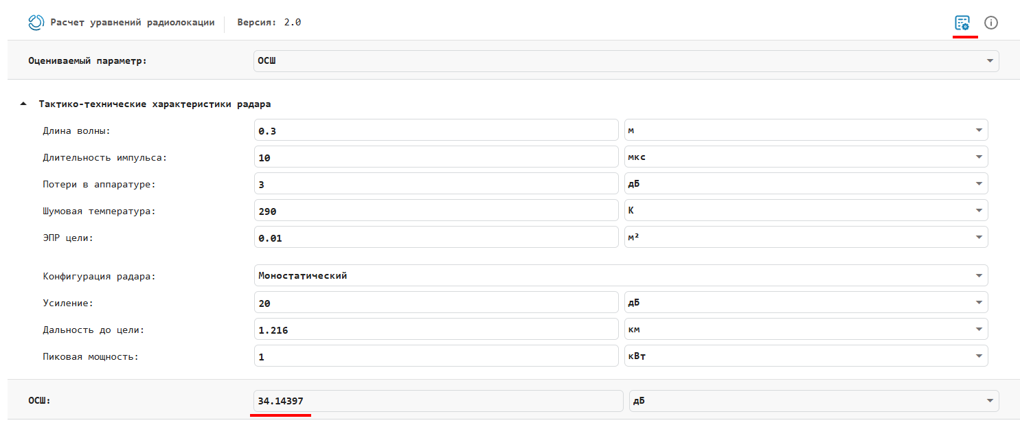
As a result, the SNR value for the current configuration was 34.1 dB. After generation, the calculation file RadarEquationScript_2026-05-29_21:46:25.749.jl appeared in the file browser. The resulting parameterized code is shown below:
tgtrng = maximum(abs_dist) # target range
# calculation of the SNR with an accuracy of 3 digits
snr = round(radareqsnr(
	lambda, # wavelength
	tgtrng, # target range
	Pt, # pulse power
	T, # pulse duration
	RCS = 0.01, # EPR of the goal (choose the average value)
	Gain = Grx, # antenna gain
	Loss = LFtx+LFrx,  # losses in the path
	Ts = TN # noise temperature
)[1];sigdigits = 3)

println("Current SNR: $snr db")
To analyze the effectiveness of the algorithm, we will select the last pulse of the signal at the receiver output and form a vector for increasing the noise power. noise_vec and SNR values snr_vec:
y = deepcopy(data_y[:,:,end]) # copying the signal data for the last pulse
ang_trues_end =  data_ang_true[:,:,end]; # copying the true directions of goals

noise_vec = collect(20:10:70) # the vector of noise power increase from 20 to 70 dB relative to NP
snr_vec = snr .- noise_vec # vector of SNR values

println("SNR vector: $(round.(snr_vec;sigdigits=3)) dB")
3.1 The MUSIC Algorithm
Consider the efficiency of the algorithm MUSIC. We will make 6 calls with MUSIC with a 10-fold decrease in SNR from call to call.:
# allocation of memory for an incomparable spectrum and angle estimates for MUSIC
spec_music = zeros(length(el_scan),length(az_scan), length(noise_vec))
ang_music = zeros(2, num_tgts, length(noise_vec)) # true directions for goals

@inbounds for i in 1:length(noise_vec)
    println("Estimation calculation for SNR $(round(snr_vec[i];sigdigits=3)) dB")
    release!(music) # resetting the system object to its initial state
    noise_sig =  sqrt(NP*10^(noise_vec[i]/10))*randn(size(y)) # new data for the noise signal
    spec_music[:,:,i],ang_music[:,:,i] = music(y.+noise_sig); # assessment of the range and directions of arrival of goals
end
Let's compare the direction finding results for the specified SNR:
fig_spec_music_vec = [] #
@inbounds for i in 1:length(noise_vec)
    push!(fig_spec_music_vec,
        plot_spec_azel(az_scan,el_scan,spec_music[:,:,i];
            title = "MUSIC (SNR = $(round(snr_vec[i];sigdigits=3)) db)"
        )
    )
end
plot(fig_spec_music_vec...)
At 24 dB, there is a confident reception of all 4 targets. As the SNR decreases, the number of detectable targets decreases: for -15.9 dB, 2 targets are visible, for -25.9 dB, target detection is lost.
Next, consider the maximum positioning error for all purposes.:
sort_ang_music = similar(ang_music) # sorted angle estimation data
[sort_ang_music[:,:,i] .= sort_ang_mse(ang_trues_end,ang_music[:,:,i]) for i in 1:length(snr_vec)]

# building a table
calc_table_ang_analysis(ang_trues_end,sort_ang_music,snr_vec)
When the SNR decreases to -16 dB, the positioning accuracy decreases for weak targets, and as the signal continues to weaken, the error becomes random.
3.2 The MVDR algorithm
Next, let's look at the efficiency of the algorithm. MVDR.
# allocation of memory for an incomparable spectrum and angle estimates for MVDR
spec_mvdr = zeros(length(el_scan),length(az_scan), length(noise_vec))
ang_mvdr = zeros(2, num_tgts, length(noise_vec)) # true directions for goals

@inbounds for i in 1:length(noise_vec)
    println("Estimation calculation for SNR $(round(snr_vec[i];sigdigits=3)) dB")
    release!(mvdr) # resetting the system object to its initial state
    noise_sig =  sqrt(NP*10^(noise_vec[i]/10))*randn(size(y)) # new data for the noise signal
    spec_mvdr[:,:,i],ang_mvdr[:,:,i] = mvdr(y.+noise_sig); # assessment of the range and directions of arrival of goals
end
Let's compare the direction finding results for the specified SNR:
fig_spec_mvdr_vec = [] #
@inbounds for i in 1:length(noise_vec)
    push!(fig_spec_mvdr_vec,
        plot_spec_azel(az_scan,el_scan,spec_mvdr[:,:,i];
            title = "MVDR (SNR = $(round(snr_vec[i];sigdigits=3)) db)"
        )
    )
end
plot(fig_spec_mvdr_vec...)
At 14 dB, there is a confident reception of all 4 targets. As the SNR decreases, the number of detected targets decreases: for -16 dB, 2 targets are visible, for -20 dB, none are visible.
Next, consider the maximum positioning error for all purposes.:
sort_ang_mvdr = similar(ang_mvdr) # sorted angle estimation data
[sort_ang_mvdr[:,:,i] .= sort_ang_mse(ang_trues_end,ang_mvdr[:,:,i]) for i in 1:length(snr_vec)]

# building a table
calc_table_ang_analysis(ang_trues_end,sort_ang_mvdr,snr_vec)
When the SNR decreases to 0 dB, the positioning accuracy decreases for weak targets, and as the signal continues to weaken, the error becomes random.
3.3 The Beamscan algorithm
Next, let's look at the efficiency of the algorithm. BeamScan.
# allocation of memory for an incomparable spectrum and angle estimates for beamscan
spec_beamscan = zeros(length(el_scan),length(az_scan), length(noise_vec))
ang_beamscan = zeros(2, num_tgts, length(noise_vec)) # true directions for goals

@inbounds for i in 1:length(noise_vec)
    println("Estimation calculation for SNR $(round(snr_vec[i];sigdigits=3)) dB")
    release!(beamscan) # resetting the system object to its initial state
    noise_sig =  sqrt(NP*10^(noise_vec[i]/10))*randn(size(y)) # new data for the noise signal
    spec_beamscan[:,:,i],ang_beamscan[:,:,i] = beamscan(y.+noise_sig); # assessment of the range and directions of arrival of goals
end
Let's compare the direction finding results for the specified SNR:
fig_spec_beamscan_vec = [] #
@inbounds for i in 1:length(noise_vec)
    push!(fig_spec_beamscan_vec,
        plot_spec_azel(az_scan,el_scan,spec_beamscan[:,:,i];
            title = "beamscan (SNR = $(round(snr_vec[i];sigdigits=3)) db)"
        )
    )
end
plot(fig_spec_beamscan_vec...)
For any SNR value (-20 to 30 dB), stable target detection is observed. At the same time, the width of the main lobes is significantly larger than for the previous algorithm, which indicates poor resolution and the inability to detect 2 close targets.
Next, consider the maximum positioning error for all purposes.:
sort_ang_beamscan = similar(ang_beamscan) # sorted angle estimation data
[sort_ang_beamscan[:,:,i] .= sort_ang_mse(ang_trues_end,ang_beamscan[:,:,i]) for i in 1:length(snr_vec)]

# building a table
calc_table_ang_analysis(ang_trues_end,sort_ang_beamscan,snr_vec)
As we can see, even with low SNR, targets are correctly detected, which indicates the high noise immunity of the algorithm.
3.4 Algorithm comparison
Let's compare the results for the selected SNR value. snr_i :
plot_spec_2d = [];
for snr_i in eachindex(snr_vec)
    spec_beamscan_snr_0db_norm = maximum(spec_beamscan[:,:,snr_i];dims=1)[:]./maximum(spec_beamscan[:,:,snr_i])
    spec_mvdr_snr_0db_norm = maximum(spec_mvdr[:,:,snr_i];dims=1)[:]./maximum(spec_mvdr[:,:,snr_i])
    spec_music_snr_0db_norm = maximum(spec_music[:,:,snr_i];dims=1)[:]./maximum(spec_music[:,:,snr_i])

    fig = plot(az_scan,spec_beamscan_snr_0db_norm,lab="BeamScan",xlab="Azimuth, degree",
        ylab="Rated power",lw=2,
        title="Comparison of direction finding algorithms for SNR = $(round(snr_vec[snr_i];sigdigits = 3)) dB"
    )
    plot!(az_scan,spec_mvdr_snr_0db_norm,lab="MVDR",lw=2,ls = :dash)
    plot!(az_scan,spec_music_snr_0db_norm,lab="MUSIC",lw=2,ls = :dashdot)
    push!(plot_spec_2d,fig)
end
plot(plot_spec_2d...;layout = (length(plot_spec_2d),1),size = (600,300*length(plot_spec_2d)))
As previously noted, the BeamScan algorithm has the worst resolution, but the best noise immunity: at -26 dB, the algorithm was able to detect the target in the direction of 6.5 degrees. The MVDR algorithm has excellent resolution with sufficient SNR (from 10 dB), but it is highly susceptible to noise. The MUSIC algorithm has the best resolution and noise immunity characteristics: even at SNR = -6 dB, confident detection of 4 targets is observed in the spatial spectrum***.***
Conclusion
Thus, in the example, the approach of modeling a multi-channel broadband direction finding system with multiple targets in the [Engee] modeling environment was considered (https://start.engee.com /).
Also, a comparative analysis of direction finding algorithms (MUSIC,BeamScan,MVDR) was performed at different values of the signal-to-noise ratio (in the range from -36 to 14 dB):
- *MVDR algorithm : shows high efficiency - high resolution at SNR values greater than zero, but is most susceptible to noise;
- algorithm Beamscan: with sufficient SNR, it has the largest width of the main lobe and, as a result, the worst resolution of the spatial spectrum. At the same time, it has the best noise immunity and is able to detect a target even at SNR< -20 dB;
- *The * Music algorithm: shows high efficiency over a wide dynamic range (-20 to 14 dB) and has the best resolution among all the presented algorithms.
Sources
- Van Treece, H. Optimal signal processing. New York: Wiley-Interscience, 2002.
- Semichastnov, A. E., and D. A. Balakin. "Modeling scenarios of a radar system for classifying unmanned aerial vehicles and birds based on Microdopler signatures in the Engee environment." Electronic Libraries, vol. 28, issue 4, November 2025, pp. 943-52, doi:10.26907/1562-5419-2025-28-4-943-952.
- A. R. Gorbunov, M. R. Akmalov, A. E. Semichastnov and D. A. Balakin, "Algorithm for Drone Recognition from Birds Based on a Neural Network Approach Using Radar Data," 2025 7th International Youth Conference on Radio Electronics, Electrical and Power Engineering (REEPE), Moscow, Russian Federation, 2025, pp. 1-8, doi: 10.1109/REEPE63962.2025.10971050.