Simulation of an automatic liquid level control system in a tank

This example demonstrates a model of a tank liquid level control system based on physical components.

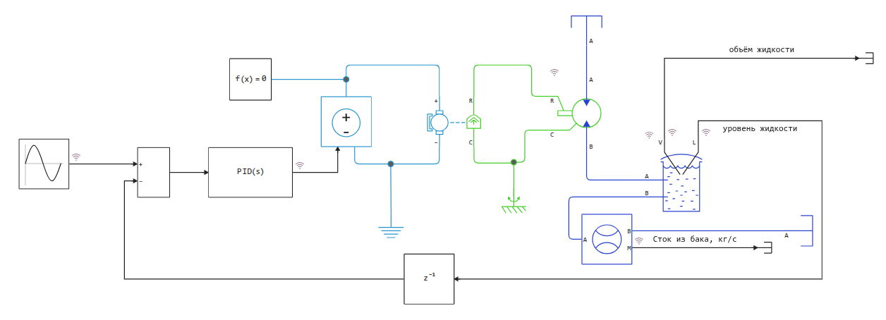
The model is a closed control loop where liquid enters the tank through a controlled pump and flows out through an outlet characterized by hydraulic resistance. The level sensor continuously measures the current height of the liquid column in the tank and transmits this signal to the control unit.

Model diagram:

Defining the function to load and run the model:

function start_model_engee()
    try
        engee.close("liquid_level_control_system", force=true) # closing the model
        catch err # if there is no model to close and engee.close() is not executed, it will be loaded after catch.
            m = engee.load("$(@__DIR__)/liquid_level_control_system.engee") # loading the model
        end;

    try
        engee.run(m) # launching the model
        catch err # if the model is not loaded and engee.run() is not executed, the bottom two lines after catch will be executed.
            m = engee.load("$(@__DIR__)/liquid_level_control_system.engee") # loading the model
            engee.run(m) # launching the model
        end
end

start_model_engee (generic function with 2 methods)

Running the simulation

start_model_engee();

Isolation of liquid level and setpoint signals from the simout variable:

result = simout;
res = collect(result);

Writing signals to variables:

level = collect(res[15])
sin_sig = collect(res[24]);
tank_mfr = collect(res[11])
pump_mfr = collect(res[25]);

Visualization of simulation results

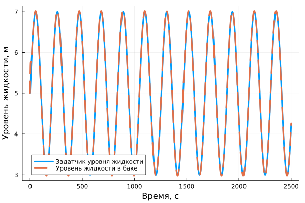
Liquid level graph and setpoint signal:

using Plots
gr()
plot(sin_sig[:,1], sin_sig[:,2], label="Liquid level sensor", linewidth=3, xlabel="Time, from", ylabel="Liquid level, m")
plot!(level[:,1], level[:,2], label="Liquid level in the tank", linewidth=3, linestyle=:dash)

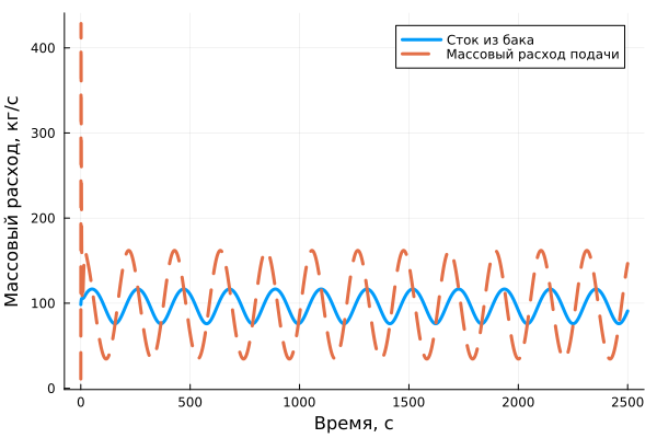
Graph of the mass flow rate of the liquid passing through the pump and through the outlet of the tank:

plot(tank_mfr[:,1], tank_mfr[:,2], label="Drain from the tank", linewidth=3, xlabel="Time, from", ylabel="Mass flow rate, kg/s")
plot!(pump_mfr[:,1], pump_mfr[:,2], label="Mass flow rate of the feed", linewidth=3, linestyle=:dash)

Conclusions:

In this example, a simulation of an automatic liquid level control system in a tank was demonstrated. Such models can be used to optimize a wide range of processes, starting with filling a water tower and ending with complex processes in the chemical industry.