Acoustic noise reduction
In this example, we will analyze the system that we control from the model and allows us to apply and filter the noise applied to the filter together with the acoustic signal.
We will use the LMS Filter block. It can implement an adaptive FIR filter using five different algorithms. The block evaluates the filter weights necessary to minimize the error.
The picture below shows the upper level of the model.
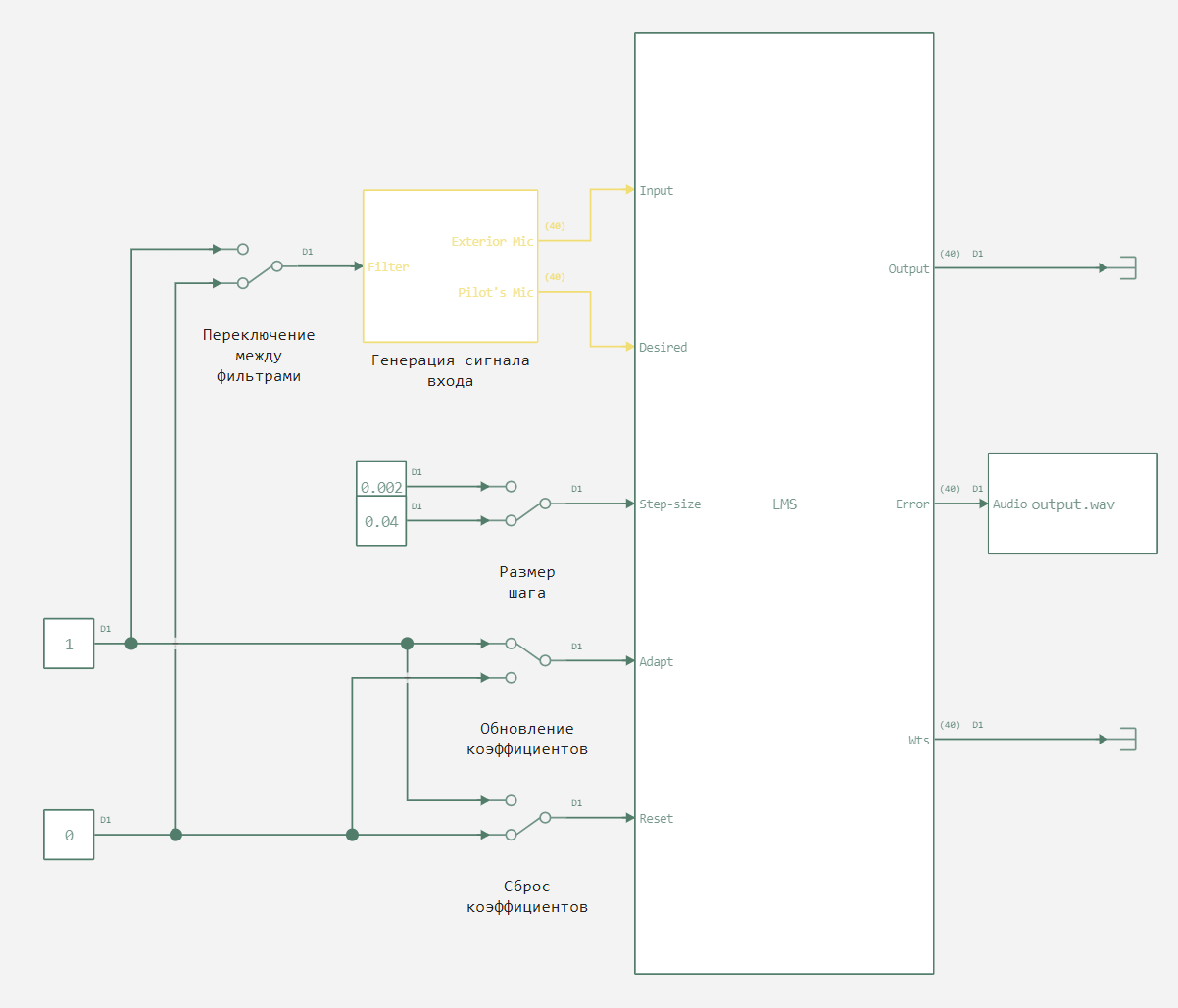
Here you can control the presence of noise in the signal, as well as filter parameters.:
- Step size,
- updating the filter weights,
- Reset the filter weights.
Now let's define auxiliary functions for working with this model.
Pkg.add(["WAV"])
# Enabling the auxiliary model launch function.
function run_model( name_model)

    Path = (@__DIR__) * "/" * name_model * ".engee"

    if name_model in [m.name for m in engee.get_all_models()] # Checking the condition for loading a model into the kernel
        model = engee.open( name_model ) # Open the model
        model_output = engee.run( model, verbose=true ); # Launch the model
    else
        model = engee.load( Path, force=true ) # Upload a model
        model_output = engee.run( model, verbose=true ); # Launch the model
        engee.close( name_model, force=true ); # Close the model
    end
    sleep(5)
    return model_output
end

# Declaring the audio player function
using WAV;
using .EngeeDSP;
function audioplayer(patch, fs, Samples_per_audio_channel);
    s = vcat((EngeeDSP.step!(load_audio(), patch, Samples_per_audio_channel))...);
    buf = IOBuffer();
    wavwrite(s, buf; Fs=fs);
    data = base64encode(unsafe_string(pointer(buf.data), buf.size));
    display("text/html", """<audio controls="controls" {autoplay}>
    <source src="data:audio/wav;base64,$data" type="audio/wav" />
    Your browser does not support the audio element.
    </audio>""");
    return s
end
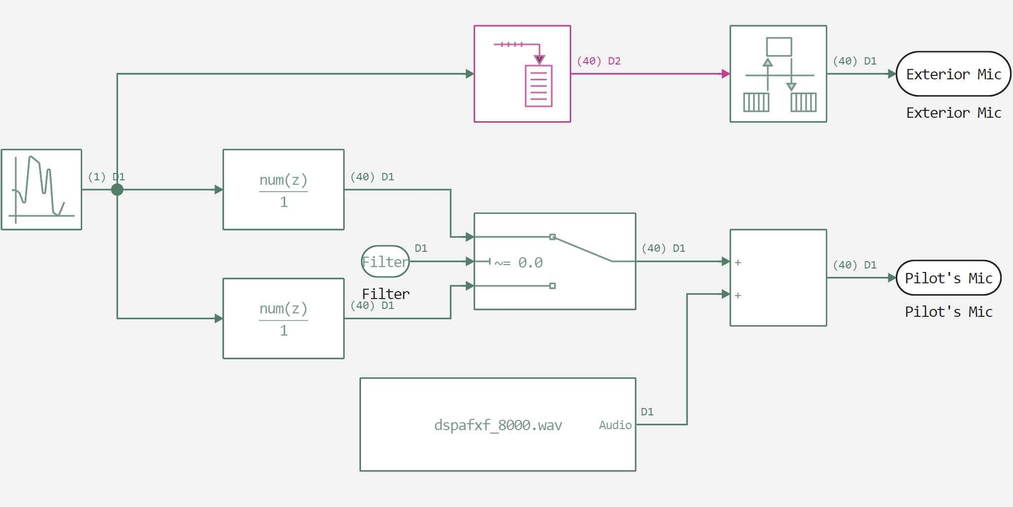
After declaring the functions, we will load coefficients for FIR filters used in the subsystem shown in the figure below from the variable file.
using FileIO
f1 = load((@__DIR__) * "/filter_values.jld2", "f1");
f2 = load((@__DIR__) * "/filter_values.jld2", "f2");
inp = audioplayer("$(@__DIR__)/dspafxf_8000.wav", 8000, 256);
Now that we have added all the necessary variables to the workspace and described the auxiliary functions, let's move on to running the model and analyzing the data obtained.
run_model("AcousticNoiseCanceler") # Launching the model.
Now let's turn to the audio player function we described earlier and play back two signals – noisy and recorded after filtering.
inp = audioplayer("$(@__DIR__)/Pilot.wav", 8000*40, 256);
out = audioplayer("$(@__DIR__)/output.wav", 8000*40, 256);
On the recording, you can hear that after filtering, the sound became clearer than before it.
using FFTW
fs = 100
gr()
plot(fftfreq(length(inp[1:2000]), fs), abs.(fft(inp[1:2000])./length(inp[1:2000])),
        xguide="Frequency  / Hz", yguide="Magnitude")
plot!(fftfreq(length(out[1:2000]), fs), abs.(fft(out[1:2000])./length(out[1:2000])),
        xguide="Frequency  / Hz", yguide="Magnitude")
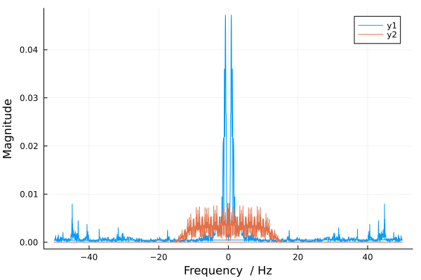
It is noticeable that the spectrum is different. The reason for the difference is that the filter significantly changes the frequency characteristics of the signal.
Let's perform an explicit comparison of the input and output data.
gr()
plot(inp[500:1000]-out[500:1000])
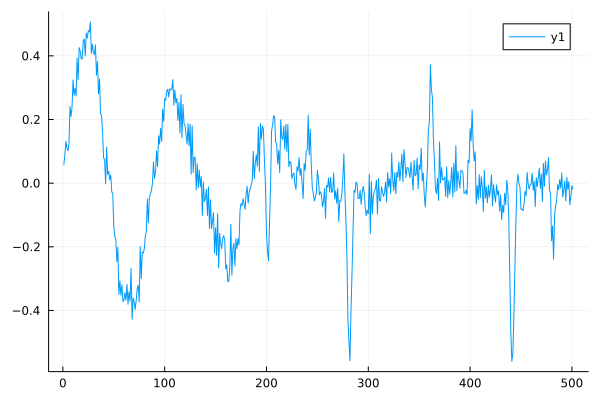
Also, when subtracting the input signal, we see significant differences in the data.
Conclusion
We have learned how to set up an acoustic noise canceller and how to change its parameters. With this model, you can do a large number of experiments by changing the filter settings and superimposed noise.