Filtering of a noisy signal by sliding averaging
This example shows how to use the block Moving RMS perform moving average filtering (simple and exponential). By changing the block settings, we will get four different types of filter behavior.
Description of the model and filters
Block Pulse Generator generates rectangular pulses with a length of 512 time samples each. Block Switch controls the switching between the upper and lower levels of the meander (between 0.5 and 1.5). We add noise to this signal with a mathematical expectation of 0 and a variance of 0.001.
For smoothing using the sliding window method (moving average (MA)) or the FIR filter, we implement two modes that differ in the overlap coefficient of the windows. In one case, the filter will jump by 1 dimension, in the other by 4 dimensions. The result of these filters will almost not differ in the value of the output value, however, the sampling of the filter with an overlap of 4 will be 4 times lower than that of the filter with a jump of 1.
We also implement a set of IIR filters with exponential smoothing (exponential moving average (EMA)).), for which we will set different weight coefficients: 0.9 and 0.99. They significantly affect the output signal: a graph with a lower smoothing coefficient (0.9) will react more dynamically to both interference and signal switching between levels.
For more information about the operation of these smoothing methods and their parameters, see the help for the [Moving RMS] block (https://engee.com/helpcenter/stable/dsp-statistics/moving-rms.html ).
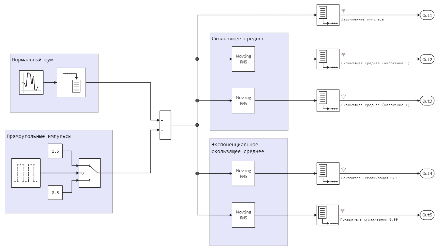
Individual areas of the model are highlighted using annotations containing SVG markup.
Sampling rate of the model
Since it is necessary to specify the step size of the model in Engee, working with multi-speed models requires careful attention to the discretization of different blocks. Let's look at one situation. The noise generator is triggered 512 times more often than the pulse generator. The model is configured to take 44,100 measurements per second.
If the first smoothing filter has a jump size of the smoothing window equal to 4, then the sampling frequency of the signal after this filter will be (512/4)/44100, that is, 128/44100 * (we can say 128 samples)*.
But if we want to make the jump size equal to 5, we will have to change the base sampling rate of the model. Indeed, at the output of such a filter, the signal will have a sampling rate of (512/5)/44100, that is, 102.4/44100 (fractional number of samples). In this case, the base sampling rate of the model is no longer the common divisor for the sampling rate of all the signals on the canvas. To restore the model's performance, it will need to be increased by 5 times (5*44100).
Launching the model
Let's run the model using software controls and compare the results of different filters.
modelName = "mvgRMSNoisyStep";
model = modelName in [m.name for m in engee.get_all_models()] ? engee.open( modelName ) : engee.load( "$(@__DIR__)/$(modelName).engee");
engee.set_param!( modelName, "StopTime"=>8 );
data = engee.run( modelName, verbose=false )
Let's build a general schedule:
plot( data["Noisy pulses"].time[1:16:end], data["Noisy pulses"].value[1:16:end],
    c=5, label="Noisy pulses" )
plot!( data["MA - The jump size is 4"].time[1:16:end], data["MA - The jump size is 4"].value[1:16:end],
    c=1, label="The jump size is 4" )
plot!( data["MA is the jump size of 1"].time[1:16:end], data["MA is the jump size of 1"].value[1:16:end],
    c=2, label="The jump size is 1" )
plot!( data["EMA - Smoothing index 0.9"].time[1:16:end], data["EMA - Smoothing index 0.9"].value[1:16:end],
    c=3, label="Smoothing index 0.9" )
plot!( data["EMA is a smoothing index of 0.99"].time[1:16:end], data["EMA is a smoothing index of 0.99"].value[1:16:end],
    c=4, label="The smoothing index is 0.99" )
Let's zoom in on the graph to see how different smoothing algorithms work out a sharp change in signal strength.
r1 = 65500:2:65800
r2 = (4*r1.start):2:(4*r1.stop)

plot( data["Noisy pulses"].time[r2], data["Noisy pulses"].value[r2],
       c=5, label="Noisy pulses" )
plot!( data["MA - The jump size is 4"].time[r1], data["MA - The jump size is 4"].value[r1],
        c=1, label="The jump size is 4" )
plot!( data["MA is the jump size of 1"].time[r2], data["MA is the jump size of 1"].value[r2],
        c=2, label="The jump size is 1" )
plot!( data["EMA - Smoothing index 0.9"].time[r2], data["EMA - Smoothing index 0.9"].value[r2],
        c=3, label="Smoothing index 0.9" )
plot!( data["EMA is a smoothing index of 0.99"].time[r2], data["EMA is a smoothing index of 0.99"].value[r2],
        c=4, label="The smoothing index is 0.99" )
Conclusion
We compared several signal averaging methods performed using the block Moving RMS With different settings, we can implement the algorithm we need, as well as objectively choose the best filtering method.