Comparison of MATLAB and Engee in spectral and time-frequency analysis problems
Comparing MATLAB and Engee in the fields of spectral analysis and time-frequency analysis, we will consider their capabilities and approaches for two tasks: forward and reverse Fourier transforms and time-frequency analysis.
Let's set a random input signal.
Pkg.add(["DSP"])
x_in = randn(300)
plot(x_in)
Spectral Fourier Transform (FFT and IFFT)
Engee uses functions from the FFTW package:
- FFT: direct fast Fourier transform.
- ifft: inverse Fourier transform.
using FFTW

# Direct Fourier transform
X = fft(x_in)

# The inverse Fourier transform
x_e = ifft(X)
MATLAB has built-in functions for fast Fourier transform:
- FFT: direct fast Fourier transform.
- IFFT: Inverse fast Fourier transform.
using MATLAB

# Direct Fourier transform
mat"""X = fft($(x_in));"""

# The inverse Fourier transform
x_m=mat"""ifft(X);"""
Let's compare the results and calculate the margin of error.
plot(x_in)
plot!(real(x_e))
plot!(x_m)
error_e = abs.(x_in-real(x_e))
error_m = abs.(x_in-x_m)
println("Average Engee error: $(sum(error_e)/length(error_e))")
println("Average MATLAB error: $(sum(error_m)/length(error_m))")
In both environments, the result of the forward Fourier transform is complex numbers, and the reverse transform returns the original signal with a small error associated with numerical rounding.
So you can see that the syntax and logic of the code are identical.
Time-frequency Fourier transform
There are no standard functions in Engee for such transformations, and they must be implemented manually.
using DSP
# A function for generating a chirp signal
function chirp(t::AbstractVector{T}, f0::T, t1::T, k::T) where T<:Real
    return cos.(2π * (f0 .* t .+ 0.5 * k .* t.^2))
end

# Hamming Window
function hamming(N::Int)
    n = 0:N-1
    return 0.54 .- 0.46 .* cos.(2π * n / (N - 1))
end

x = chirp(0:0.001:1, 0.0, 1.0, 100.0)  # Chirp signal
l=500 # Window size
window=vcat(hamming(l),zeros(length(x)-l))

P = DSP.periodogram(x; fs=1000, window=window, nfft=length(x))

# Visualization of the spectrum
plot(freq(P), 20*log10.(power(P)), xlabel="Frequency (Hz)", ylabel="Power Spectrum (dB)", title="Power Spectrum", linewidth=2)
MATLAB has a pspectrum function that allows you to perform time-frequency analysis of a signal.
pspectrum automatically selects the appropriate analysis method.
Supports various visualizations (spectrograms, power densities).
using Images
mat"""cd("$(@__DIR__)")"""
mat"""
% Time-frequency analysis
x = chirp(0:0.001:1, 0, 1, 100);
pspectrum(x, 1000); % Time-frequency spectrum
saveas(gcf, 'frequency_time_spectrum.jpg'); % Сохраняет текущую фигуру как JPG
"""
load( "$(@__DIR__)/frequency_time_spectrum.jpg" )
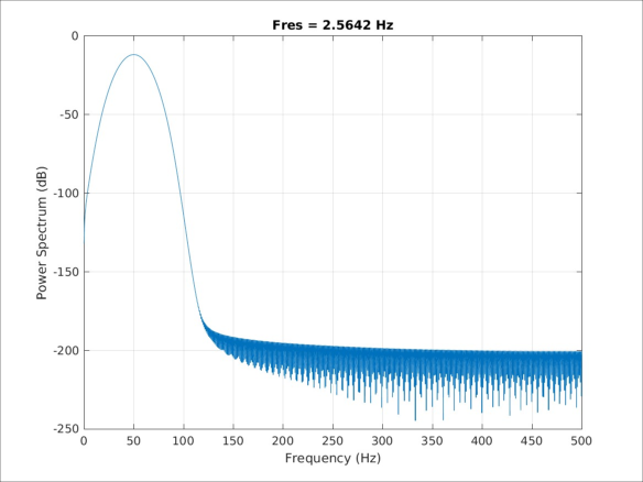
Based on the graphs, it can be seen that the main trends in signal behavior are reflected in Engee. For more detailed plotting, it is necessary to additionally implement a more detailed calculation of the window for the periodogram function.
Also, let's compare the correctness of the generated input data in MATLAB and Engee.
plot(mat"chirp(0:0.001:1, 0, 1, 100)"[:])
plot!(chirp(0:0.001:1, 0.0, 1.0, 100.0))
title!("Sum_error: $(sum(mat"chirp(0:0.001:1, 0, 1, 100)"[:]-chirp(0:0.001:1, 0.0, 1.0, 100.0)))")
As we can see, the input signals are identical.
Conclusion
MATLAB has built-in functions for performing these operations. In Engee, you can use third-party libraries for this task, such as DSP or FFTW for more complex signal operations. It is also important to consider that Engee provides more flexibility in how transformations can be implemented. To simplify these operations for your Engee tasks, use the ready-made approaches described in this demo.
Another aspect in comparing the capabilities of the two environments suggests that MATLAB is optimized for working with matrices and signals. However, Engee is generally faster in computing if the code is written taking into account the specifics of this environment, and this gives a significant increase in the speed of execution and testing algorithms in large systems.