Polyphase sampling frequency converter
In this example, the application of the FIR Rate Conversion block is analyzed.
This unit performs an efficient polyphase
conversion of the sampling frequency
using a rational coefficient.
L/M along the first dimension.
The block treats each column of the input
signal as a separate channel and resamples
the data in them independently of each other.
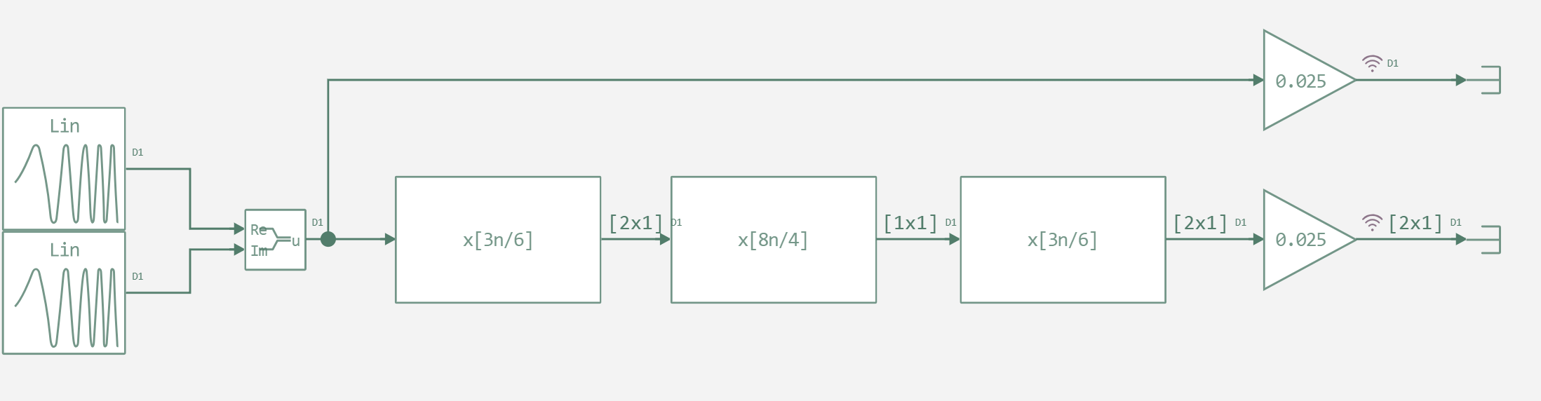
Now let's look at the model itself, developed
for this example. It generates a complex signal,
to which a polyphase conversion of the sampling frequency is applied.
Auxiliary functions
# Enabling the auxiliary model launch function.
function run_model( name_model)

    Path = (@__DIR__) * "/" * name_model * ".engee"

    if name_model in [m.name for m in engee.get_all_models()] # Checking the condition for loading a model into the kernel
        model = engee.open( name_model ) # Open the model
        model_output = engee.run( model, verbose=true ); # Launch the model
    else
        model = engee.load( Path, force=true ) # Upload a model
        model_output = engee.run( model, verbose=true ); # Launch the model
        engee.close( name_model, force=true ); # Close the model
    end
    sleep(5)
    return model_output
end

using FFTW
# Calculation of the signal spectrum
function compute_spectrum(signal, fs)
    n = length(signal)
    spectrum = abs.(fft(signal)) / n
    freqs = (0:n-1) .* (fs / n)
    spectrum[1:Int(n/2)], freqs[1:Int(n/2)]  # Return half of the spectrum (for convenience)
end
Launching the model and analyzing the calculation
In this example, the filter coefficients will be taken from a MAT file pre-recorded for this model.
Pkg.add("MAT")
using MAT
# Reading data from a .mat file
file = matopen("$(@__DIR__)/Hm.mat")
var_names = names(file)
print("$var_names")

for var_name in var_names
    value = read(file, var_name)# Getting the value of a variable from a file
    @eval $(Symbol(var_name)) = $value # Dynamic creation of a variable named var_name
end
# Closing the file
close(file)
run_model("Rate_Conversion") # Launching the model.
Now let's compare the input and output data.
inp = collect(simout["Rate_Conversion/inp"])
sim_time = vcat([m[] for m in inp.time]...)  # Extracting values from matrices
inp = vcat([m[] for m in inp.value]...)  # Extracting values from matrices

out = collect(simout["Rate_Conversion/out"])
out = vcat([vec(m2) for m2 in out.value]...)  # Convert each matrix into a vector

println("Number of input encoded data: $(length(inp))")
print("Number of output encoded data: $(length(out))")
As we can see, the output contains 2 times more values
than the input. This indicates that
interpolation has been performed – the process of increasing the sampling frequency of a signal
by adding new samples between existing ones.
gr()
A = plot(real(inp[1:1000]), imag(inp[1:1000]), seriestype=:scatter, legend=false,
     xlabel="Re", ylabel="Im", title="Entrance")
B = plot(real(out[1:1000]), imag(out[1:1000]), seriestype=:scatter, legend=false,
     xlabel="Re", ylabel="Im", title="Exit")
plot(A,B)
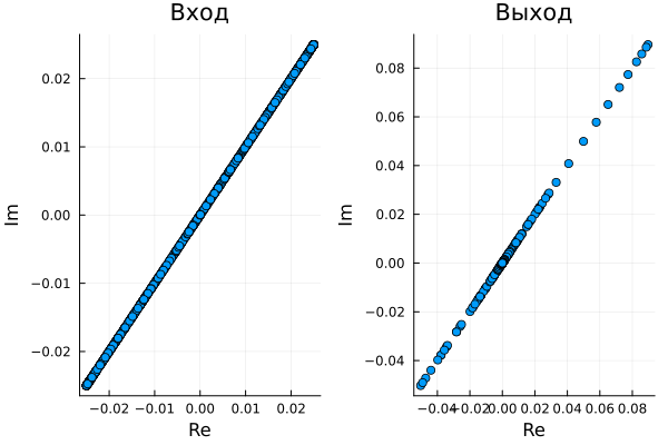
Based on the results of data visualization, it can be seen
that the amplitude of the distribution of values at the output
differs significantly from the values at the input.
Now let's look at the results of the spectral comparison of the input and output.
spectrum_inp, freqs_inp = compute_spectrum(inp[1:4000], 1000)
spectrum_out, freqs_out = compute_spectrum(out[1:4000], 1000)
plot(
plot(freqs_inp, spectrum_inp, xlabel="Frequency (Hz)", ylabel="Amplitude", title="Entrance", label=""),
plot(freqs_out, spectrum_out, xlabel="Frequency (Hz)", ylabel="Amplitude", title="Exit",  label="")
)
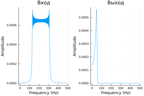
This comparison showed that the signal spectrum was significantly
distorted, and the useful signal was lost after the transformations, based on the
results of spectral analysis.
Conclusion
In this demonstration, we examined a polyphase
sampling frequency converter and the possibilities of using it to change
the sampling frequency of a signal. This option will be very useful for your projects.