Signal averaging
How to implement the simplest method of signal averaging using basic blocks? Let's look at the example of a simple model of how to divide the accumulated amount by the number of elements in the sample and get the arithmetic mean of the input signal.
Description of the model
The simplest way to average a signal is to sum all the available elements and divide the sum by the number of elements in the vector. If we receive a signal at the input , then the sequence of output signals such a filter should be as follows:
The diagram contains the summation blocks (Sum) and taking the previous value (Delay). The upper half of the model is responsible for calculating the numerator in the above expressions, summarizes the input elements. The lower part of the model summarizes the constant 1 as many times as the simulation steps have been completed.
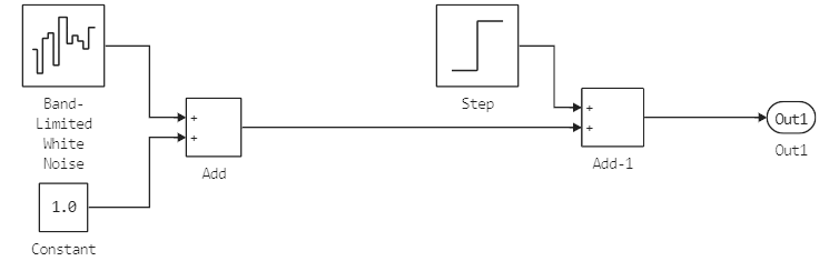
The signal that we are averaging is simply the result of summing a constant 1 with a vector of uniformly distributed noise with amplitude 0.01. After 500 samples of the model, an amplitude step is added to the signal. 1.
.png)
Launching the model
Let's run the model using software management tools.
# If the model is not open yet, we will download it from the file
if "running_average" ∉ getfield.(engee.get_all_models(), :name)
    engee.load( "$(@__DIR__)/running_average.engee");
end;

data = engee.run( "running_average" )
plot(
    plot( data["The original"].time, data["The original"].value, label="The original signal", legend=:bottomright),
    plot( data["Smoothed out"].time, data["Smoothed out"].value, label="Smoothed signal", legend=:bottomright ),
    layout=(2,1)
)
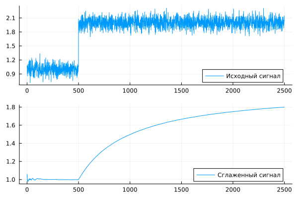
The advantage of this type of filtering is the quick initial setting of the filter: after starting the model, the output signal overcame the distance from 0 to 1 in a few couple of samples and stabilized after several dozen simulation cycles.
The disadvantage, as we can see, is a very slow response to subsequent changes. The longer the signal history, the slower the filter output value will respond to the step.
Conclusion
We have implemented a simple signal averaging method, which is very easy to implement in the form of graphical blocks or in the form of code for processing simulation results.