Smoothing the signal with a sliding window
Let's consider 4 ways to smooth the signal with a sliding window, from low-level to the highest-level.
Different ways to smooth the signal
In different applications, an engineer may need a variety of signal filtering methods, and we will analyze four methods (which work identically) and discuss their advantages and disadvantages.
Chain of delays (explicit FIR)
First, the lowest-level method of implementing a sliding window would be to simply store a certain number of signal points, for example 100, as they arrive. The result will be the sum of all these "deferred measurements" divided by their number (100).
.png)
There are 10 identical blocks inside the filter, the outputs of which are summed and divided by 100.
.png)
There are 10 delay blocks inside each such block. Unit Delay, which store the next value before passing to the next block the value they received a step earlier.
Why did we create such a hierarchy of blocks? By arranging the delay blocks in this way, we avoided the need to create a line of 100 delay blocks.
This method is not very flexible, since we still have to create delay blocks manually. It will be difficult to parameterize such a filter using a mask.
Using a ready-made FIR filter unit
It is much easier to place a block on the diagram. Discrete FIR filter
.png)
We will specify the same weights of coefficients for the block, so that each measurement has the same contribution to the final signal.
Smoothing through the CIC filter
A FIR filter with the same weights can be created using a much simpler and more elegant design shown below.
.png)
Here, using a delay length of 100 and a few simple blocks, we have created a cascaded integrated comb filter of the BIH type (with infinite impulse response). There are no multiplication operations at all, so the filter works very fast.
The "Moving Average" block
Another block from the standard library is called Moving Average if the "sliding window" method is specified in its settings, it will implement the same operation as the previous ones.
The block needs a vector of values to come to its input, so we send a buffered signal to the input port (block Buffer length 100 with overlap 99). At the output, it will return us a single value packed into a matrix of size 1х1. We will convert it to a scalar using the block Demux.
Launching the model
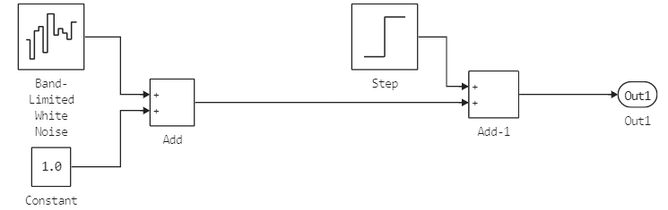
Let's run the model for 2500 counts. The input signal is generated by the following subsystem:
.png)
This is the result of summing the constant 1 with a vector of uniformly distributed noise with amplitude 0.01. After 500 samples of the model, an amplitude step is added to the signal. 1.
# If the model is not open yet, we will upload it from the file
if "moving_average" ∉ getfield.(engee.get_all_models(), :name)
    engee.load( "$(@__DIR__)/moving_average.engee");
end;

data = engee.run( "moving_average" )
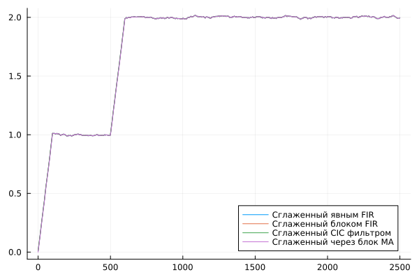
Let's compare the results with each other. They should be identical, but the latter method will introduce a delay of one count due to the way the buffering of the signal is implemented.
plot( data["Smoothed by explicit FIR"].time, data["Smoothed by explicit FIR"].value, label="Smoothed by explicit FIR" )
plot!( data["Smoothed by the FIR block"].time, data["Smoothed by the FIR block"].value, label="Smoothed by the FIR block" )
plot!( data["Smoothed by a CIC filter"].time, data["Smoothed by a CIC filter"].value, label="Smoothed by a CIC filter" )
plot!( data["Smoothed through the MA block"].time, data["Smoothed through the MA block"].value, label="Smoothed through the MA block" )
plot!( legend=:bottomright )
Conclusion
If you often have to filter signals in your work, then it will be useful for you to work with the models presented in this example.
The choice of filter depends on whether you need to set weights (for example, implement an exponential filter), as well as on which signal comes to the input (scalars or vectors) and whether you need to translate the model into code or not.