Equalization of time-shifted signals
Often, during measurements, data is received asynchronously from different sensors. To make a cumulative picture when using multiple sensors, the data needs to be synchronized.
For this application, we will need the DSP library for digital signal processing and the FileIO library for uploading JLD2 files.
Pkg.add( ["DSP", "JLD2"] )
Let's read the input data and plot the graphs.:
using JLD2
@load "relategsignals.jld2"

plot(
    plot( s1, label=L"s_1" ),
    plot( s2, label=L"s_2" ),
    plot( s3, label=L"s_3" ),
    layout=(3,1), link = :x
)
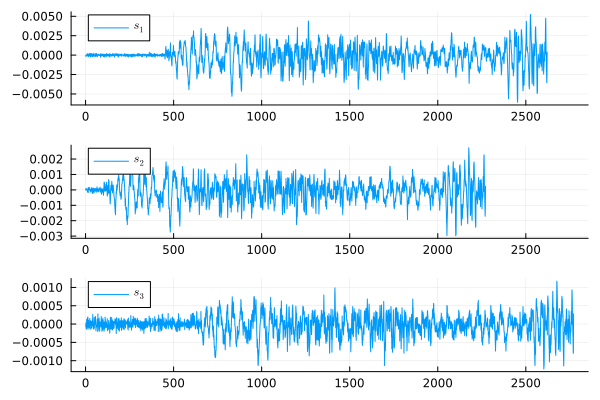
As we can see, the signal s2 comes before s1, and s1, in turn, is ahead of s3. The exact delay between signals of the same length can be found using the function DSP.Util.filddelay and to apply it to signals of different lengths, we will reduce the length of all signals to the length of the smallest of them.
As a result, we will notice that s2 ahead of the signal s1 at 350 counts, that s3 It's relatively late s1 for 150 counts, and also that the signal s2 ahead of s3 for 500 counts.
using DSP

min_size = min( size(s1,1), size(s2,1), size(s3,1) )
t12 = DSP.Util.finddelay(s1[1:min_size], s2[1:min_size])
t31 = DSP.Util.finddelay(s3[1:min_size], s1[1:min_size])
t32 = DSP.Util.finddelay(s3[1:min_size], s2[1:min_size])

t12, t31, t32
Align the signals manually relative to s2 (who arrives before everyone else):
plot( s1[t12+1:end], label=L"s_1", size=(600,300) )
plot!( s2, label=L"s_2" )
plot!( s3[t32+1:end], label=L"s_3" )
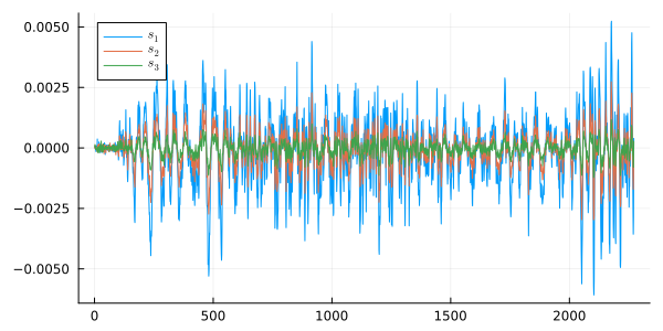
Units have been added to the offset, because at offset 0, you need to output a signal starting at index 1. It would be easier to use the function DSP.Util.shiftsignal.
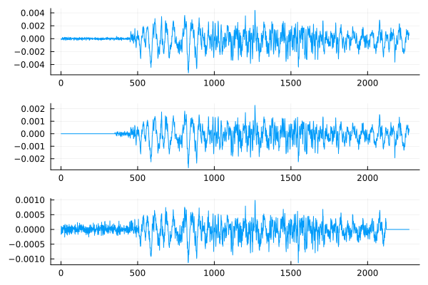
The function will allow us to avoid intermediate operations. alignsignals. It delays earlier signals, so that all signals will be shifted by the time the signal arrives. s3.
x1 = s1[1:min_size]
x2,t21 = DSP.Util.alignsignals( s2[1:min_size], s1[1:min_size] )
x3,t31 = DSP.Util.alignsignals( s3[1:min_size], s1[1:min_size] );

plot(
    plot( x1 ),
    plot( x2 ),
    plot( x3 ),
    layout=(3,1), leg=false
)
Conclusion
Now the studied signals are synchronized in time of occurrence and we can proceed with further processing.