Implementation of a FIR filter on basic elements
In this example, we will analyze the structure of the FIR filter and analyze the behavior of the filter at different coefficients within it.
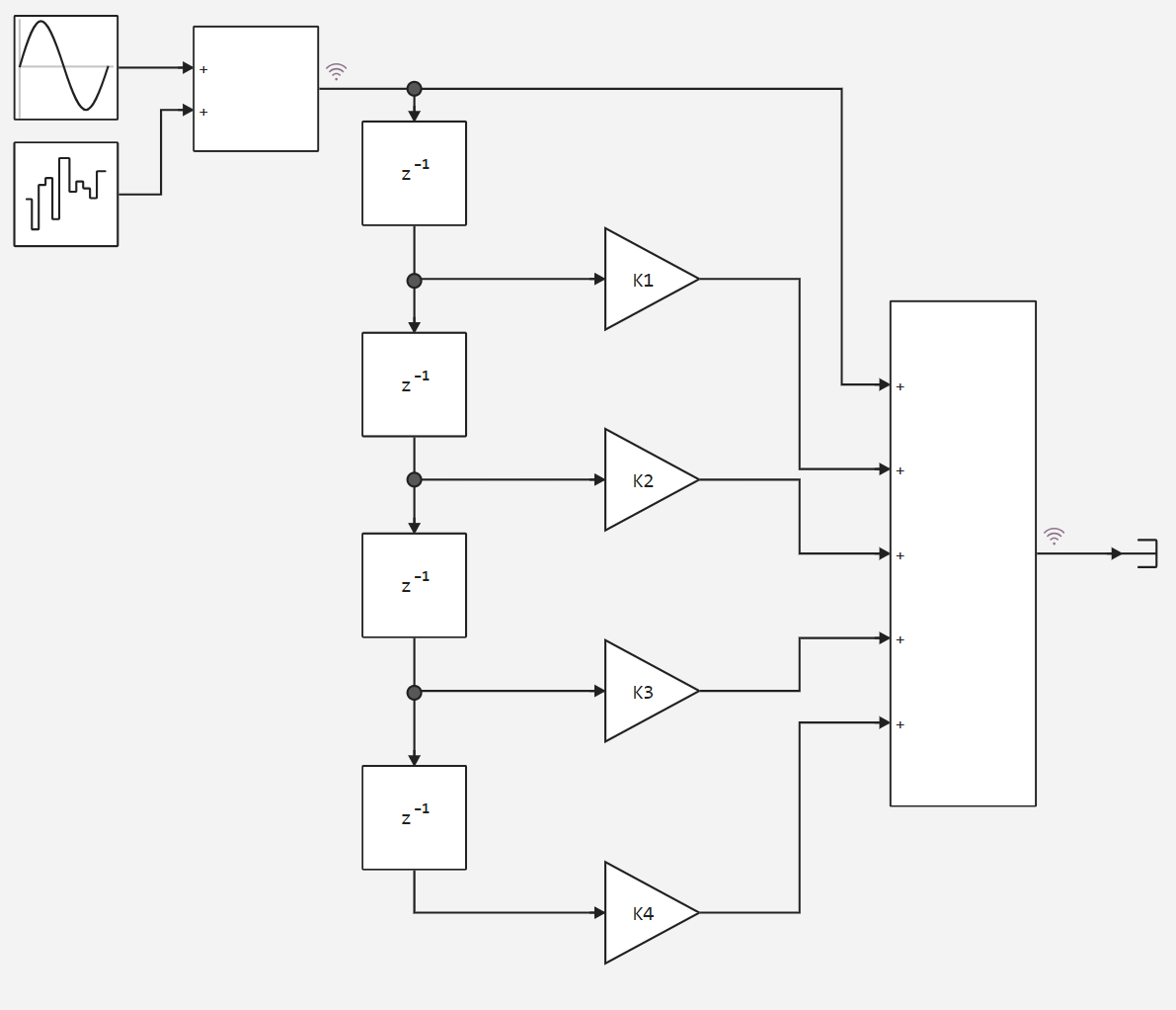
The basic filter consists of a delay line and coefficients by which the delayed signal is multiplied, after which the results are added together.
The figure below shows the FIR filter circuit containing 4 coefficients.
Next, we add an auxiliary function of the model and determine the coefficients for several filter runs.
In [ ]:
# Enabling the auxiliary model launch function.
function run_model( name_model)

    Path = (@__DIR__) * "/" * name_model * ".engee"

    if name_model in [m.name for m in engee.get_all_models()] # Checking the condition for loading a model into the kernel
        model = engee.open( name_model ) # Open the model
        model_output = engee.run( model, verbose=true ); # Launch the model
    else
        model = engee.load( Path, force=true ) # Upload a model
        model_output = engee.run( model, verbose=true ); # Launch the model
        engee.close( name_model, force=true ); # Close the model
    end
    sleep(5)
    return model_output
end
Out[0]:
In [ ]:
K_agg = [0.1 0.2 0.3 0.4; 0.16 0.38 0.38 0.16; 1 2 3 4]
Out[0]:
Let's run the model in a loop, and analyze the results by plotting graphs in the time and frequency domains.
In [ ]:
out_arr = zeros(1001,3)
K, K1, K2, K3, K4 = 0, 0, 0, 0, 0
for i in 1:3
    K = K_agg[i,:]
    K1, K2, K3, K4  = K[1], K[2], K[3], K[4]
    run_model("Basic_FIR_filter") # Launching the model.
    out = collect(simout["Basic_FIR_filter/out"]);
    out_arr[:,i] = out.value
end

plot(out_arr)
Out[0]:
In [ ]:
using FFTW

Comp_out = ComplexF64.(out_arr);
spec_out = fftshift(fft(Comp_out));

plot([10log10.(abs.((spec_out/3e6)))], label =["0.1 0.2 0.3 0.4" "0.16 0.38 0.38 0.16" "1 2 3 4"])
ylabel!("Power DBW")
xlabel!("Frequency MHz")
Out[0]:
Conclusion
As we can see from the resulting graphs, the filter coefficients affect changes in both signal power and frequency characteristics.