Wavelet transformation of signals with the construction of a scalogram
The wavelet transform is a powerful signal analysis tool that allows you to study time and frequency characteristics simultaneously. This method is particularly useful for processing nonlinear and non-periodic signals such as biological data, financial series, and acoustic signals. One of the most popular applications of wavelet analysis is the construction of scalograms, which are two-dimensional graphs showing the distribution of signal energy over time and frequency.
For example, consider the problem of analyzing a composite signal consisting of two cosine components and random noise. The signal announcement will be performed in Engee and the resulting analysis will also be performed on MATLAB to compare the capabilities of these two environments.
Pkg.add(["ContinuousWavelets", "Wavelets"])
fs = 1000 # Sampling rate
t = 0:1/fs:1-1/fs # Time vector
signal = cos.(2π*50*t) .+ cos.(2π*120*t) .+ randn(length(t))  # Composite signal with noise
plot(t, signal)
To implement such an analysis in Engee, we will need the following libraries:
- ContinuousWavelets
- Wavelets
- FFTW
Pkg.add("Wavelets")
Pkg.add("ContinuousWavelets")
using ContinuousWavelets, Wavelets, FFTW
Let's analyze in detail the code described below.
wavelet is a function that creates a waveform converter object. In our case, it takes three arguments:
- Morlet(π) is the Morlet wave function with parameter π. The Morlet function is widely used in signal analysis due to its ability to efficiently identify signal features at different scales.
- averagingType=NoAve() — defines the type of averaging. No averaging is selected here. This means that each point in the resulting array will correspond to the value of the wave coefficient without additional smoothing.
- β=2 is a parameter that determines the window width of the Morlaix function. The higher the β value, the narrower the window and the more accurate the localization of the signal in the time domain, but the worse the resolution in the frequency domain.
CWT — This function performs continuous wave transformation (CWT) of the original signal using a built-in wave converter.
c = wavelet(Morlet(π), averagingType=NoAve(), β=2)
res = cwt(signal, c)
heatmap(abs.(res)', xlabel= "time",ylabel="frequency")
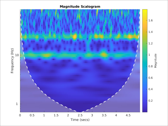
Now let's build the same thing in MATLAB. In this case, cwt differs in syntax and calculates the coefficients of the wave transformation for the input signal and the number of scales. It is also important to clarify that a larger number of scales provides a more detailed analysis, but requires more computing resources.
using MATLAB
mat"""
cwt($(signal),200);
saveas(gcf, 'Wavelet.jpg'); % Сохраняет текущую фигуру как JPG
"""

load( "$(@__DIR__)/Wavelet.jpg" )
Conclusion
The graphs showed that the results are identical in both environments.