Generation and analysis of vector signals

Introduction

In this basic example, we will look at the principle of generating
vector signals using the example of five discrete sinusoids,
learn about the basic operations on vector signals,
and also get acquainted with the possibilities of their visualization
in the time and frequency domains.

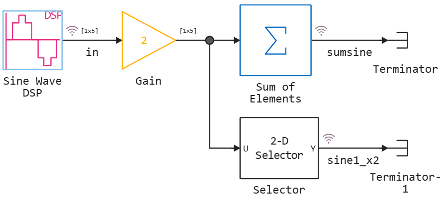
The model consists of blocks of a discrete sinusoidal signal source DSP Sine Wave,
block Gain, multiplying the input signal by a constant value,
block Sum of Elements, summing the elements of the vector input,
and the block Selector, which extracts elements from the vector input.

Generating multiple sinusoids

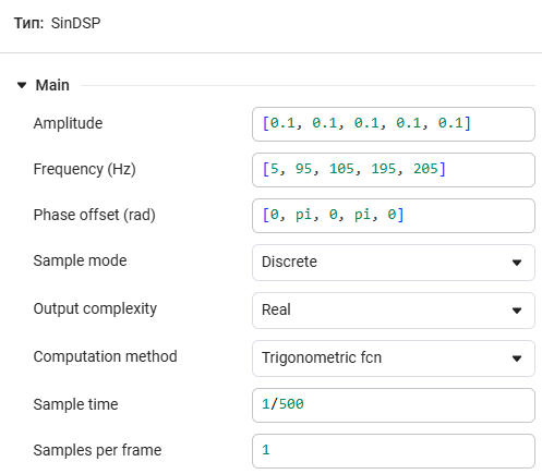
The parameters of the signal source block are shown in the figure below.
It is worth noting that in the model we generate five sinusoids at once,
setting the values of amplitudes, frequencies and initial phases using a vector.
In our case, we generate signals of the same amplitude at
frequencies of 5 Hz, 95 Hz, 105 Hz, 195 Hz and 205 Hz.
Moreover, the initial phase changes 180 degrees from
a sine wave to a sine wave.
The sampling frequency of the signal is 500 Hz.

We could observe a similar composition of the frequency components of a complex
periodic signal in the example
Multi-speed Filter,
where their superposition resulted in a waveform with outliers
and zeros in between. In the current example, we will try
to reproduce a similar waveform.

The spectrum of vector and total signals

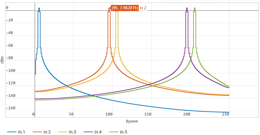
Let's display the spectrum of the signal in in the window Графики by selecting
in Меню сигналов: Сигналы в частотной области.
We observe five spectra of five discrete sinusoids
at the indicated frequencies:

Now let's consider the spectrum of the total signal at the output
of the block Sum of Elements. We see the spectrum of a single signal,
but its peaks are at the same frequencies.:

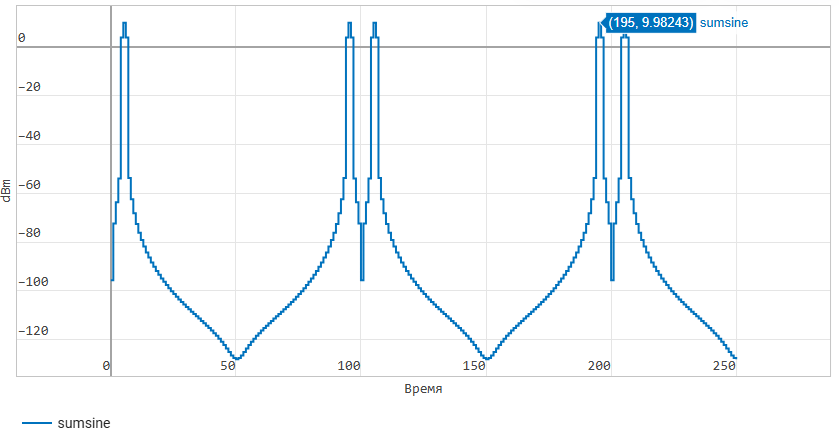
It can be noted that the power level of the peaks in the spectrum of the total signal
is higher than that of the peaks of individual sinusoids by 6 dB. This is due
to the fact that we pass a vector signal through the block. Gain,
doubling the amplitude of each of the vector elements.
The multiplication operation is vectorized, at the output of the block Gain the signal is also
vector-based.

Time domain signal visualization

Now let's build waveforms of the signal in by selecting
in Меню сигналов: Сигналы во временной области.
We observe five discrete sinusoids
with different repetition periods on the same axes. We can also disable individual vector elements on the legend
below the graph, displaying the signals we are interested in.

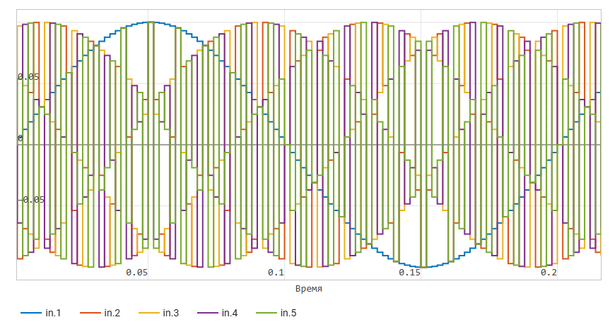
The amplitude of each of the sinusoids at the output of the signal generator is 0.1.
After the block Gain The range of the sinusoids becomes from -0.2 to 0.2.

The shape of the resulting signal

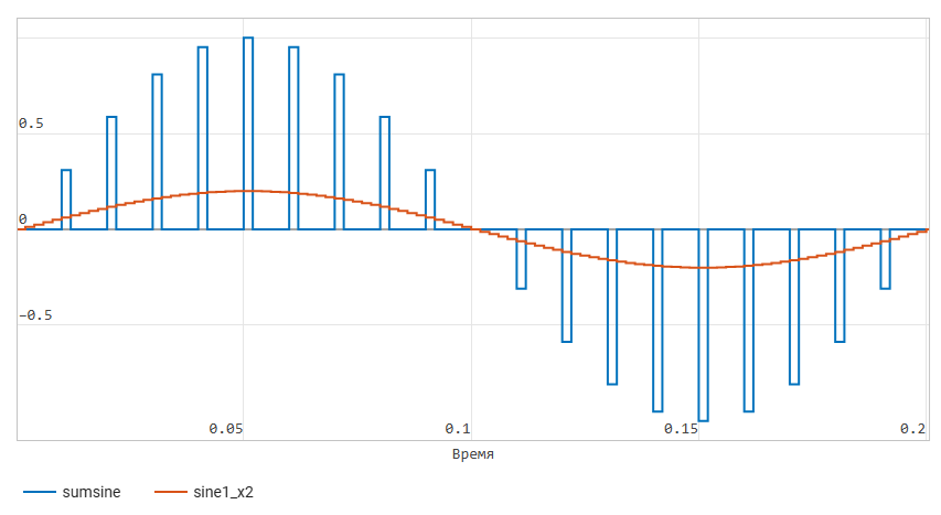
If we reflect the waveform at the output
of the block in the time domain Sum of Elements, the expected waveform can be observed.
These are pulse emissions of sinusoid samples ranging from -1 to 1
with dips to zero between emissions. When five discrete sine
waves with an amplitude of 0.2 are added in phase, we get the maximum of the total
signal, but most often their superposition gives zero.:

You can also output one of the sinusoids from the output of the block to the graph.
Gain In this case , we use the block Selector to
extract a single scalar signal from a vector. In the model
, the first element of the vector is allocated, that is, a sine wave with an amplitude of 0.2
and a frequency of 5 Hz.

Conclusion

In this model, using the example of a source of five sinusoids, we got acquainted
with the principles of generating vector signals, displaying them in
time and frequency domains, performing vectorized
arithmetic operations on vector signals,
operations on an array (using the example of the sum of array elements),
and selecting individual elements of a vector signal.