Multirate filter¶

Introduction¶

Multirate systems are discrete systems containing signals with different sampling rates (SR) are called multirate systems. In most cases, systems that vary the sampling rate of the input signal are considered. It can be increased and decreased by an integer number of times, as well as changed by a fractional number of times (m/n, where m and n are integers). On the example of this model we will consider the classical problem of changing the PD by a fractional number of times, and also learn why we need a filter.

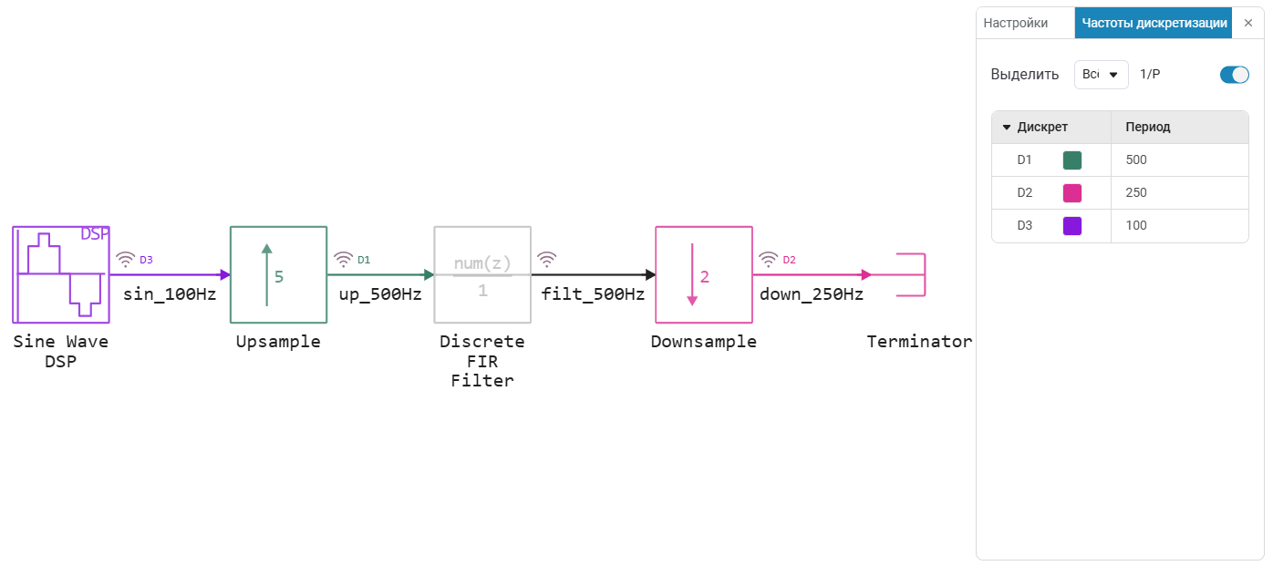
The model consists of the discrete sinusoidal signal source block DSP Sine Wave, the block of increasing PD by an integer factor Upsample, the block of decreasing PD by an integer factor Downsample, and the filter block Discrete FIR Filter, which is initially inactive (the signal passes through the block without changes). The original discrete sinusoid is a signal with a fundamental frequency of 5 Hz and a sampling frequency of 100 Hz. Block Upsample increases the PD by a factor of 5 in a very simple way - by adding four extra zeros between the samples of the incoming sinusoid. The Downsample block thins the samples of the incoming signal by removing (in our case) every second sample. Thus we want to increase the PD of the sinusoid by 2.5 times. On the Отладка tab in the model we highlight the PD of blocks and signals with different colours.

Running the model and output waveform¶

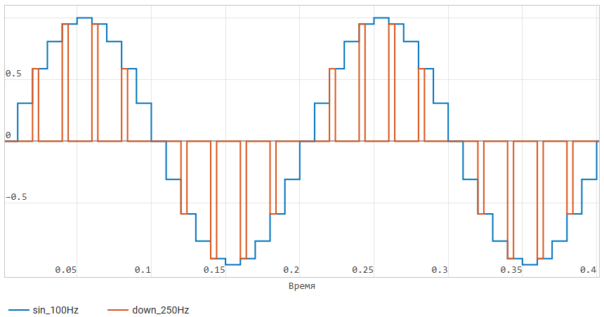
When we run the model for simulation, we can observe in the window Графики signals in the time domain. Note that the original signal looks like a discrete (stepped) sinusoid, while the model output (a signal with a PD of 250 Hz) is an emission with zeros between them. the output of the model (250 Hz PD signal) is an emission with zeros in between.

Blocks Upsample and Downsample - implement simple digital algorithms that change PD. But they do not perform interpolation and decimation in the usual sense.

To understand how the block helps in such operations. Discrete FIR Filter let's first look at what happens to the spectrum of the signal as the PD is raised and lowered.

Spectral copies and aliasing when changing the sampling rate¶

To do this, let's use the built-in interactive tool for visualisation of the signal spectrum in the window Графики, by selecting in Меню сигналов: Сигналы в частотной области. Successively we will display the signals (it is important to realise that for a correct display signals must have the same sampling frequency on the same axes).

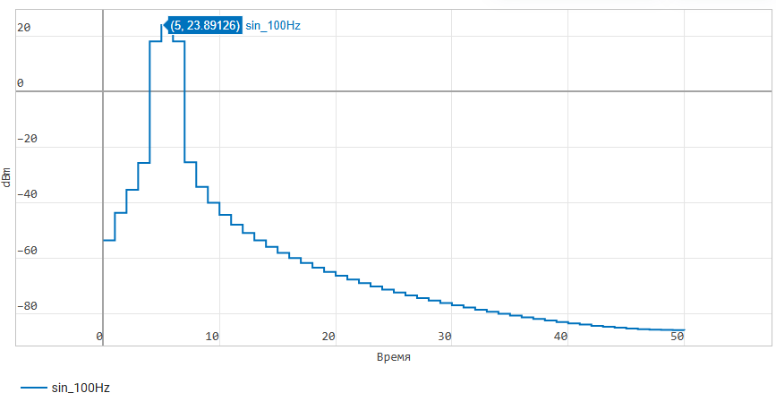
First, we will display the spectrum of the original discrete sinusoid. Let's make sure that the peak of the spectrum is at 5 Hz, and the X-axis of the graph lies between 0 and 50 Hz (i.e. up to half of the sampling frequency):

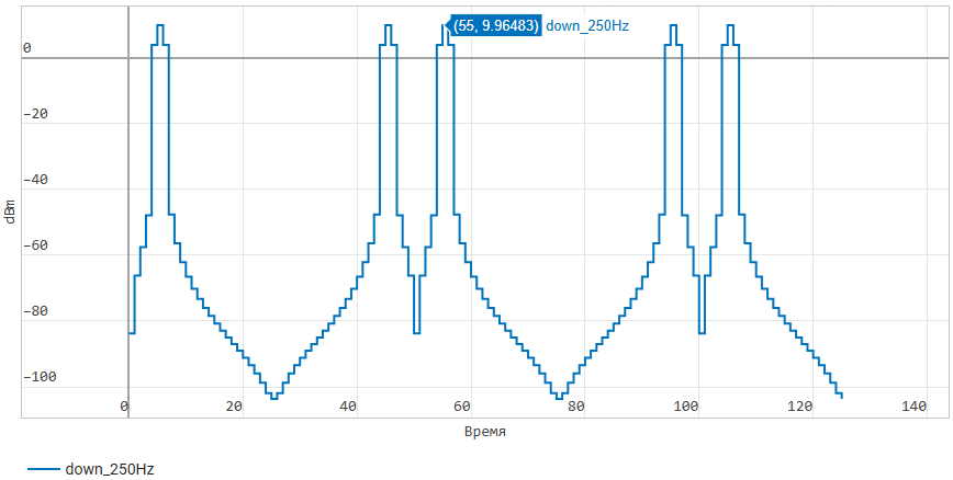
Now let us consider the signal spectrum after increasing the PD by a factor of 5:

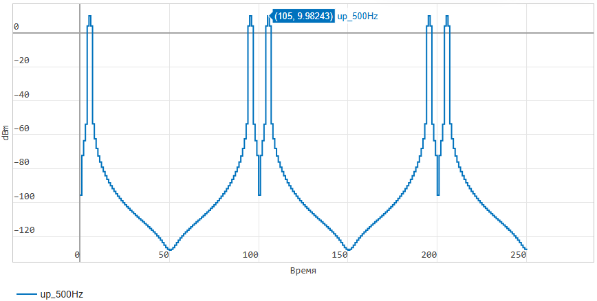
The spectrum of a discrete signal is inherently periodic, and as we expand the Nyquist zone of frequency observation to a new value of half the PD, we start to see spectral copies of our signal. In our case, sinusoids are seen at frequencies of 5 Hz, 95 Hz, 105 Hz, 195 Hz, 205 Hz.

And when we further narrow the spectrum after surgery. Downsample these copies are "wrapped" into a new Nyquist zone, which is now limited to 125 Hz. This is the aliasing effect:

It's the presence of spectral copies in the output signal that determines its shape - emissions with zeros. In essence, this is a complex periodic signal formed by the sum of basic signals - sinusoids. We can't eliminate them completely, but we can suppress them them with the right low-pass filter. This filter is called an anti-imaging or anti-aliasing filter. It is always placed after the operation Upsample and before the the operation Downsample.

Designing a low-pass filter¶

Our task is to develop a suitable prototype (specification) of the of the filter and put its coefficients in the block Discrete FIR Filter.

Taking into account that the original signal can lie in the range of 0 to 50 Hz, we choose a filter cutoff frequency of 50 Hz, the Kaiser window function, the normalised width of the of the transition band, as well as the required suppression in the fence band. Also note that the specification we choose is for a sampling rate of 500 Hz, since this is the signal that enters the filter input:

using DSP;
fs = 500;
mywindow = FIRWindow(; transitionwidth=0.15, attenuation=60, scale=true);
myFIR = digitalfilter(Lowpass(2*50/fs), mywindow);

We now calculate and display the amplitude-frequency response (AFR) of the amplitude-frequency response (AFR) of the filter to verify its ability to suppress spectral copies above 50 Hz:

myTransferFunction = PolynomialRatio(myFIR,1);
H, w = freqresp(myTransferFunction);
freq_vec = fs*w/(2*pi);
plot(freq_vec, pow2db.(abs.(H))*2, linewidth=3,
     xlabel = "Частота, Гц",
     ylabel = "Амплитуда, дБ",
     title = "АЧХ фильтра нижних частот",
     ylim = (-120, 10))

A 50th order filter was synthesised using the chosen specification. The shape of its frequency response, although it does not perfectly pass all frequencies of interest. frequencies of interest, but for the current task - suppression of the interfering ones - it is suitable. The coefficients of the filter coefficients are already included in the model block, so we don't have to transfer them unnecessarily.

Applying a low-pass filter¶

In the model, we right-click on the filter block and select Включить блок. After that we run the model again for simulation, and look at the spectrum of the two signals - at the input and output of the of the filter:

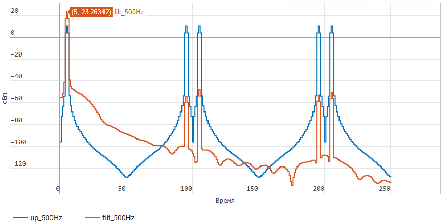
As we can see, the spectral copies are suppressed relative to the 5 Hz sinusoid by more than 70 dB. It can also be seen that the 5 Hz sine wave in the output signal has a higher higher power. We purposely multiply the filter coefficients by 5, because adding zeros with the Upsample operation reduces the energy of the signal by a factor of 5.

Now let's take a look at the shape of the output signal in the time domain:

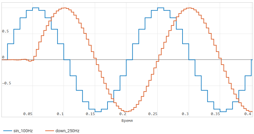
It corresponds in amplitude to the input signal, it also has a a fundamental frequency of 5Hz, its sampling rate is 250Hz, and its waveform is now a sine wave.

But we can also see that it's delayed relative to the input signal by a quarter of a period. This is the effect of using a FIR filter that's 50 samples long. 50 samples - such filters are bound to introduce delay.

Conclusion¶

In this example, we have looked at the basic principles of changing the frequency of sampling frequency in digital devices, the effects of imaging and aliasing, the necessity of using low-pass filters.