Application of system objects in signal processing
The EngeeDSP library contains powerful tools for signal processing using system objects, which are specialized components for streaming data processing. The code below demonstrates a comprehensive approach to signal processing that combines EngeeDSP system objects with traditional signal processing functions.
Let's list the key features of the implementation.
- Using the system object
SineWaveDSPto generate a signal with configurable parameters (amplitude, frequency, calculation method). - Application
DescretFIRFilterto filter the signal in streaming mode. - Integration with the usual processing functions (rolling average via convolution).
- Combining EngeeDSP's object-oriented approach with Julia's procedural methods.
Let's start by connecting the libraries used in this project.
# Pkg.add("DSP")
# Pkg.add("Statistics")

using DSP
using EngeeDSP
using Statistics
Now let's perform initialization. The code below creates a system object. SineWaveDSP from the EngeeDSP library for generating a sinusoidal signal with the specified parameters: amplitude A = 0.8, frequency f = 100 Гц, sampling rate fs = 1000 Гц, the size of the frame framesize = 796 Counts.
The object is configured for the tabular calculation method (Table lookup), real output (Real) and continuous generation mode (Continuous).
A = 0.8
f = 100
fs = 1000
framesize = 796

H = EngeeDSP.SineWaveDSP(
    Amplitude = A,
    Frequency = f,
    SampleTime = 1//fs,
    SamplesPerFrame = framesize,
    ComputationMethod = "Table lookup",
    OutputComplexity = "Real",
    SampleMode = "Continuous"
)
The code below creates a system object DescretFIRFilter, which is an FIR filter with a basic default configuration, and has the following characteristics:
CoefSource=Dialog parameters— coefficients, in this case it is an array [0.5 0.5], which corresponds to the simplest averaging filter.FilterStructure=Direct form— The standard direct filter implementation structure is used.InputProcessing=Elements as channels— Each input sample is processed as a separate channel.InitialStates=0— the initial state of the filter is zero.ShowEnablePort=falseandExternalReset=None— The filter operates continuously without external reset control.
This object is designed for streaming signal processing and stores the internal state (PreEmphasis_states=[0.0]) between calls.
fir_filter = EngeeDSP.DescretFIRFilter()
The following shows the creation of a confidant averaging filter with a window of 10 samples. Array averaging_filter filled with values 1/window_size (i.e. 0.1), which means evenly weighing all 10 previous values of the signal. This filter suppresses high-frequency noise, smoothing the signal by averaging over a given window. Unlike the EngeeDSP system objects, it is a static convolution that does not save state between calls.
window_size = 10
averaging_filter = ones(window_size) / window_size
Now let's build a model from our objects. The code below performs cyclic signal generation and processing in 100 steps:
- Signal generation:
- At every step
H()generates a new sine wave frame (lengthframesize=796counts) through the system objectSineWaveDSP.
- At every step
- Filtering:
y_fir = fir_filter(x)— applies a streaming FIR filter (with coefficients[0.5, 0.5]) to the signal, saving the state between calls.y_avg = conv(y_fir, averaging_filter)[1:length(y_fir)]— additionally smoothes the signal with moving averages (a window of 10 samples), trimming the result of the convolution to the original length.
- Saving the results:
- Source (
s), filtered (fir_filtered) and smoothed (avg_filtered) the signals are accumulated in arrays for subsequent analysis.
# Generating and processing the signal
s = Float64[]          # The original signal
fir_filtered = Float64[] # After the FIR filter
avg_filtered = Float64[] # After averaging

for n in 1:100
    x = H()
    y_fir = fir_filter(x)
    y_avg = conv(y_fir, averaging_filter)[1:length(y_fir)] # Truncate to the original length

    append!(s, x)
    append!(fir_filtered, y_fir)
    append!(avg_filtered, y_avg)
end
Now we will use the saved data to build graphs.
gr()
n_show = 100
t = (0:n_show-1)/fs

p_signals = plot(t, s[1:n_show], label="The original signal", linewidth=2)
plot!(t, fir_filtered[1:n_show], label="After FIR", linewidth=2, linestyle=:dash)
plot!(t, avg_filtered[1:n_show], label="After averaging", linewidth=2, linestyle=:dot)
title!("Signals at different stages of processing")
xlabel!("Time (s)")
ylabel!("The amplitude")
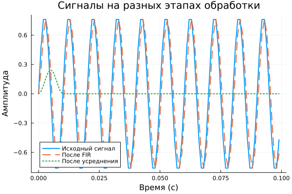
Chart results:
- The original signal (solid line) is a pure sine with an amplitude of 0.8.
— After FIR (dotted line) is a smoothed signal with reduced sharp fluctuations (the effect of the window 2 reference). - After averaging (points), the first 10 points show an increase in the average signal (the filter is "filling up"), and then zeroing, since
convit is trimmed to the length of the input signal without filling the edges.
** Why zeros?**
The moving average requires window_size-1 additional counts for complete overlap. In the code conv it is cut strictly to length y_fir discarding the "incomplete" sections of the convolution — hence the zeros after the 10th point, the zero values after averaging - is an artifact of processing, not the real behavior of the system. For streaming averaging, it is better to apply DSP.filt(averaging_filter, y_fir) with a saved state.
s = Float64[]
fir_filtered = Float64[]
avg_filtered = Float64[]

for n in 1:100
    x = H()
    y_fir = fir_filter(x)
    y_avg, filt_state = DSP.filt(averaging_filter, y_fir)

    append!(s, x)
    append!(fir_filtered, y_fir)
    append!(avg_filtered, y_avg)
end

p_signals = plot(t, s[1:n_show], label="The original signal", linewidth=2)
plot!(t, fir_filtered[1:n_show], label="After FIR", linewidth=2, linestyle=:dash)
plot!(t, avg_filtered[1:n_show], label="After averaging", linewidth=2, linestyle=:dot)
title!("Signals at different stages of processing")
xlabel!("Time (s)")
ylabel!("The amplitude")
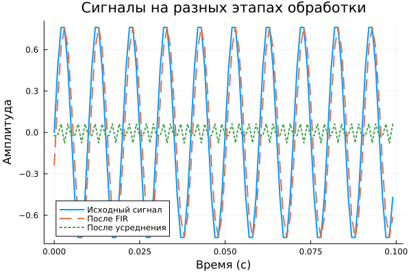
Switching to filt I eliminated the clipping artifacts, and the graph now reflects the true behavior of the system, and it also allowed us to create a fully streaming processing system where:
- FIR filter (sample window 2) smoothly smooths the signal (dotted line);
- The moving average (window of 10 samples) now correctly processes the entire signal without zeros.;
- The phase shift between the filters has become predictable, as both filters operate in stateful streaming mode.
Conclusion
The example clearly demonstrates the advantages of the combined approach, where EngeeDSP system objects are used for streaming processing, and traditional functions are used for additional transformations. The final graph is particularly indicative, which allows you to track changes in the signal at each stage of the model. Using Engee system objects in combination with traditional Julia methods opens up wide possibilities for creating efficient and flexible signal processing systems.