Adaptive signal filtering using the LMS algorithm in Engee
Adaptive filtering is a powerful digital signal processing tool that allows you to automatically adjust the filter parameters according to the changing characteristics of the input signal or the environment. Unlike static filters with fixed coefficients, adaptive filters change their parameters in real time to achieve optimal performance.
The Least Mean Squares Algorithm (LMS) is one of the most popular adaptive filtering algorithms due to its simplicity of implementation and computational efficiency. In this article, we will look at the practical implementation of the LMS filter in Engee using the EngeeDSP package.
The principle of operation of the adaptive filter
The adaptive filter consists of two main components:
- Digital filter (usually FIR-type)
- Adaptive algorithm for updating filter coefficients
The LMS algorithm minimizes the average squared error between the desired signal and the filter output. The basic equation of updating weights:
w(n+1) = w(n) + μ·e(n)·x(n)
where:
- w(n) is the vector of filter weights at step n
- m is the adaptation step (determines the rate and stability of convergence)
— e(n) is the error (the difference between the desired and actual output) - x(n) is the vector of input samples
Key parameters of the LMS algorithm
- Filter length: determines the number of coefficients and, consequently, the complexity of the model
- Adaptation step (µ): affects convergence rate and stability
- Leakage coefficient: prevents unlimited growth of coefficients
Now that we have figured out the theoretical component of this demonstration, let's look at our example of implementing an LMS filter in Engee and start by connecting libraries and initializing the filter.
Pkg.add("DSP")
using EngeeDSP, DSP
Fs = 44100  # Sampling rate
x = 0.05 * randn(1024*10)  # Input signal (white noise)
d = filt(FIRFilter([0.5, -0.3, 0.2, 0.1, -0.05]), x)  # The desired signal
HA = EngeeDSP.LMSFilter(
    Algorithm = "LMS",
    FilterLength = 32,
    StepSize = 0.1,
    LeakageFactor = 1.0,
    InitialValueOfFilterWeights = 0,
    AdaptPort = false,
    ResetPort = "None",
    OutputFilterWeights = true
)
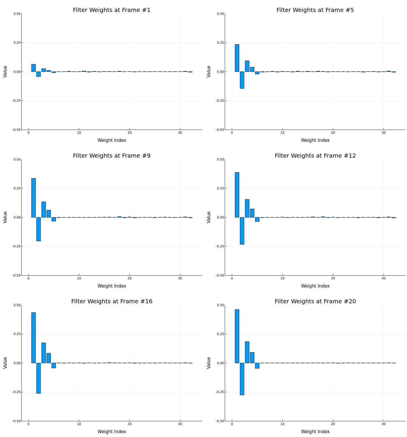
The code block shown below performs:
-
Splitting the signal into frames of 500 samples each
-
Sequential processing of each frame with updating of the filter weights
-
Visualization of weight changes in the form of an animated GIF
# Frame-by-frame signal processing
frameSize = 500
num_frames = length(x) ÷ frameSize
setup!(HA, x[1:frameSize], d[1:frameSize])

# Creating animation of changing weights
anim = @animate for i in 1:num_frames
    start_idx = (i-1)*frameSize + 1
    end_idx = i*frameSize
    y_frame, e_frame, w = step!(HA, x[start_idx:end_idx], d[start_idx:end_idx])

    bar(w, title="Filter Weights at Frame #$i",
        ylims=(-0.5, 0.5), legend=false,
        xlabel="Weight Index", ylabel="Value")
end
gif(anim, "weights_animation.gif", fps=5)
Conclusion
The presented implementation of the LMS filter in Engee demonstrates the power and flexibility of the language for digital signal processing tasks. The EngeeDSP package provides a user-friendly interface for working with adaptive filters, and built-in visualization tools make it easy to analyze the results.
The key advantages of this approach are:
- Easy to implement: complex mathematical algorithms are encapsulated in ready-made functions
- Performance: Engee provides speed comparable to C with convenient high-level syntax
- Visualization: the ability to create visual animations of the adaptation process
Adaptive filtering has applications in many fields.:
- Suppression of noise and echo in audio systems
- Highlighting useful signals against the background of interference
- Time series forecasting
- Identification of systems
Further development of this example may include:
- Comparison with other algorithms (NLMS, RLS)
- Analysis of the influence of parameters on convergence
- Application to real signals (audio, biomedical data, etc.)
