The Hilbert Filter
The Hilbert filter is a linear electronic (or digital) filter that performs a 90° phase shift** for all frequencies of the input signal without changing its amplitude. From most of the filters that we considered in other examples, we required ** frequency selectivity**, that is, amplification or attenuation of the signal in certain bands, while the Hilbert filter should behave like an ideal phase shifter.
Key concepts:
-
The output of the Hilbert filter is the Hilbert transform of the input signal
-
The Hilbert filter ** does not change the amplitude** of the signal at any frequency (ideal case)
-
FIR or BIH filters with approximate characteristics are used for implementation.
-
The combination of the original signal and its Hilbert transform makes it possible to obtain an analytical signal - a complex signal consisting of the original real signal and quadrature as the imaginary part
The Hilbert filter is widely used in DSP tasks, but in our example we will specifically consider its use to isolate the envelope of a periodic discrete signal.
Prototype of the Hilbert filter
We synthesize the coefficients of the required filter using the method remez. Our prototype will have a length of 65 samples. Let's display the impulse response (i.e. vector samples Num):
using DSP
myHBT = remez(65, [(0.05, 0.95) => 1]; Hz = 2, neg=true);
Num = reverse(myHBT);
plot(Num, line=:stem, marker=:circle, linewidth = 2, legend = false,
    title = "Impulse response of the Hilbert filter")
We see the inverse symmetry of the coefficients, as well as alternating zeros in the samples - a typical type of characteristic for Hilbert filters with an odd number of samples.
Now let's calculate and display the frequency response and frequency response of the filter. We plan to use it for signals with a sampling frequency of 5000 Hz.:
myfilt = PolynomialRatio(Num,1);
H, w = freqresp(myfilt);
freq_vec = 5000*w/(2*pi);
plot(freq_vec, pow2db.(abs.(H))*2, linewidth=3,
     xlabel = "Frequency, Hz", legend = false,
     ylabel = "Amplitude, dB",
     title = "Frequency response of the Hilbert filter",
     ylim=(-30,5))
phi, w = phaseresp(myfilt);
plot(freq_vec, rad2deg.(phi), linewidth = 3,
    xlabel = "Frequency, Hz", legend = false,
    ylabel = "Phase, degree",
    title = "Frequency response of the Hilbert filter")
The frequency response is linear over a wide frequency range, and the frequency response also does not distort the amplitude, almost covering the entire first Nyquist zone (from 0 to 2500 Hz). However, approaching the upper or lower limit, the filter will not work as efficiently, which we will notice in the simulation in the dynamic model.
The Hilbert filter model
Consider the dynamic model Hilbert_filter.engee:
It contains:
-
an amplitude-modulated sinusoidal signal source unit with a choice of carrier frequency (the modulation frequency is always 10 Hz)
-
FIR filter block with coefficients of the prototype Hilbert filter
Num -
compensating delay line of 32 counts (ntaps -1 / 2)
-
a block for generating a complex signal from the signals of the real and imaginary parts
-
the unit for calculating the modulus of a complex number
Simulation with default model parameters
By running the model, you can observe the waveforms in the graph window. real, imag and mag. The latter is responsible for calculating the envelope of the analytical signal. With a carrier frequency of 200 Hz, the signals look like this:
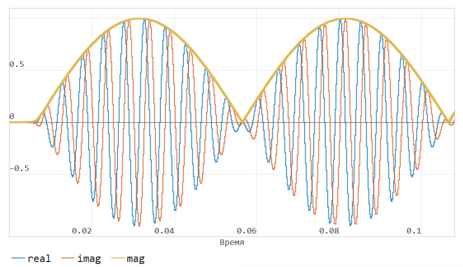
We can observe the formation of a quadrature component (with a 90-degree shift relative to the original actual signal), as well as the smooth shape of the analytical signal module, i.e. envelope.
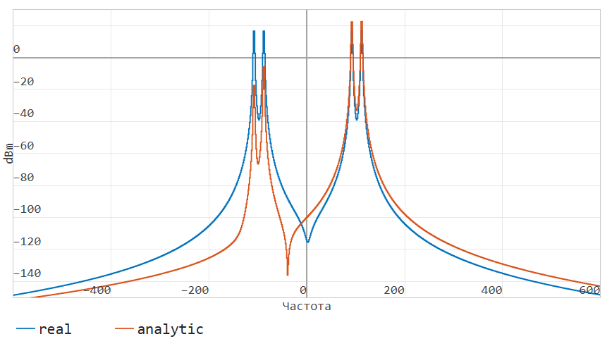
Scrolling through the graph window below, you can see a comparison of the actual and analytical signals in the frequency domain:
.png)
The actual signal peaks at frequencies of - 210 Hz, -190 Hz, 190 Hz and 210 Hz. Pay attention to the effective suppression of the negative frequency range by the Hilbert filter for the analytical signal.
Changing the frequency of the signal source
The signal source in the model allows you to quickly change the carrier frequency using a mask with a drop-down list:
.png)
If you change the value to 100 Hz and run the simulation, you can make sure that as you approach the lower limit of the FIR filter bandwidth, the shape of the envelope begins to distort:
.png)
If you need to expand the effective bandwidth, you will have to increase the filter order.
In the frequency range, it is also possible to observe a less effective suppression of the negative frequencies of the analytical signal.:
.png)
Well, for a signal with a 500 Hz carrier, there will be no such distortion, since it is in the frequency response region, which does not distort the amplitude.
Conclusion
We examined an example of an analysis of a prototype Hilbert filter, as well as a dynamic model based on a FIR implementation, an approximation operating in a limited frequency band.