FFT and spectral analysis with EngeeDSP

We continue to get acquainted with the functionality of the EngeeDSP library using the example of spectral analysis and the application of the fast Fourier transform (FFT) function.

The example is based on data from previously published projects (FFT, Spectral Analysis) which were performed using Julia plug-in libraries, such as DSP.jl, FFTW.jl, Statistics.jl and so on. In this case, there is no need to connect these libraries, since their functionality is covered by EngeeDSP.

The application features of the function are discussed below. fft to evaluate the amplitude and phase spectra of the test signal, as well as the practical task of spectral analysis to determine the characteristics of the recorded audio signal.

The FFT function

Information about the frequency and phase composition of the signal can be obtained by switching from the time domain of analysis to the frequency domain using the Fourier transform method. As a basic test signal, we will generate the sum of four sinusoids with different amplitudes, fundamental frequencies, and initial phases.:

Let's apply the function to the signal fft directly and visualize the result:

The graph is drawn on a complex plane, since the complex vector at the output of the FFT contains information about both the amplitude of the components and the phase. It is also worth noting that the number of complex samples at the output of the algorithm corresponds to the number of samples of the signal in the time domain at its input.

Let's display the module of the complex vector at the output of the FFT:

Function fftshift from the EngeeDSP composition, it allows you to represent the FFT output in the usual form of a spectrum, in our case symmetrical with respect to the center - zero frequency. But we will also have to shift the vector of discrete frequencies along the abscissa axis in the range from before :

Finally, in order to obtain the amplitude spectrum of the signal, we need to take into account the number of samples at the output of the FFT function, and also take into account that the energy of the real signal also extends to the region of negative frequencies, which, in our case, is uninformative. Let's display the amplitude spectrum of the signal in the positive frequency range using a linear graph, making sure that the amplitudes of the sinusoids are calculated correctly at the synthesized frequencies.:

Let's construct the phase spectrum of the test signal by determining the "angle" of the FFT samples by the function angle. We will mark the frequency components we are interested in with markers, make sure that the phase is calculated correctly.:

Setting the task for analysis

Let's take an audio recording of a guitar string as a signal for analysis. The main task is to determine which note is being played by analyzing the spectrum of the signal. Let's load the numerical samples of the signal with the function wavread, which also allows you to select the sampling frequency of the signal fs - in our case, it is equal to 8000 Hz:

Let's calculate the number of samples of the signal in the time domain, calculate the time step, and form a time vector and a numerical vector of samples of the signal. sig:

We'll use an additional function to listen to audio. audioplayer:

Let's listen to the sound of an oscillating string:

Let's display fluctuations in the time domain:

It is possible to find out the fundamental oscillation frequency by the shape of a periodic signal in the time domain, but it is still very difficult.

Estimation of the signal spectrum

Let's construct the audio signal power spectrum using the sequence of operations applied above. We will also evaluate the spectrum using the FFT method, but this time we will limit the number of points at the output of the function. fft 8000 counts.

Further steps repeat the standard algorithm - calculation of the complex FFT, shift, normalization by level. But to display along the ordinate axis, the square of the amplitude, i.e. the power, is already taken and converted to decibels.:

We observe an audio signal power spectrum ranging from -4,000 Hz to 4,000 Hz.

A harmonic structure is clearly visible on the spectrum - equidistant peaks. Harmonics are sinusoidal oscillations whose frequencies are multiples of the fundamental frequency. ​.

- the lowest frequency in the signal (the first harmonic), and the higher harmonics are frequencies of the form ​, where (second, third, etc.).

Determination of the fundamental frequency

By analyzing harmonics, it is possible to determine the fundamental frequency in the signal spectrum. But first, let's write a custom spectrum estimation function based on the algorithm used. As additional input arguments, it will accept the sampling frequency of the signal, the number of FFT samples, and the "one-way" spectrum flag.:

Let's analyze the low frequency range (from 0 to 1500 Hz). We will find the ** peaks** in the spectrum - they correspond to the harmonics of the signal. The function will help us with this. findpeaks from the set of EngeeDSP functions. Let's highlight the first six harmonics - these are peaks of at least -50 dB and with a severity of at least 30 - and display them on the graph.:

The very first peak is at 219 Hz. But we can also programmatically determine the frequencies of the first six harmonics and find the average distance between them in Hz. It is this estimate that we will take as the fundamental frequency.:

The fundamental frequency is calculated statistically as the arithmetic mean of the difference between the frequencies of neighboring peaks.:

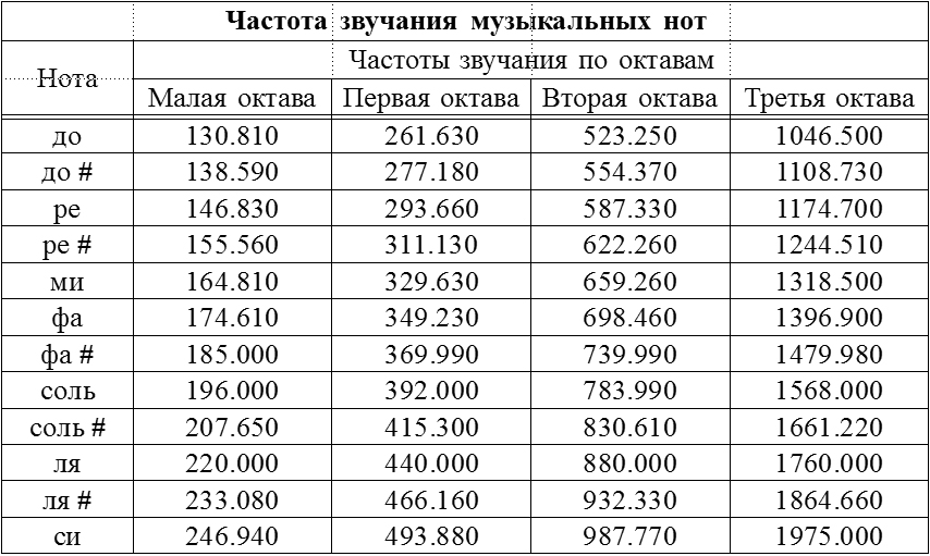
According to the table, the note played is A minor octave La.

Conclusion

We got acquainted with the EngeeDSP functionality for calculating the fast Fourier transform and implementing an algorithm for estimating the signal spectrum based on it, and solved the practical problem of determining the characteristics of an audio signal using spectral analysis.