Multi-speed processing with EngeeDSP
Multi—rate Signal Processing (Multirate Signal Processing) is a field of digital signal processing (DSP) that deals with systems where different parts of the processing process operate at different sampling rates (BH).
Simply put, it is ** a change in the sampling rate of a signal** (the number of samples per second) inside a digital system. Most often, the change is made to save computing resources (with an excessively high sampling rate of the signal), compatibility of standards (for example, audio 44.1 kHz and 48 kHz), the implementation of polyphase filters, and so on.
The main operations are increasing and decreasing the sampling rate by an integer number of times. Their combination also allows you to change the BH in a fractional number of times (, where and - whole ones).
In this example, we will consider the functions from the EngeeDSP library used for the task of increasing the BH signal by 2.5 times (interpolation), and also note the importance of using low-pass filters (low-pass filters) in the practical implementation of such systems.
include("helper.jl") # enabling a set of additional functions
Test signal for processing
As a test signal, we will generate one sinusoid of the main frequency of 100 Hz with a sampling frequency of 2 kHz. The task is to increase the sampling frequency of the sine wave by 2.5 times, that is, raise it 5 times and then halve it.
fs = 2000;                  # sampling rate of the signal
f0 = 100;                   # the main frequency of repetitions of the sine wave
dt = 1/fs;                  # time grid step
t = 0:dt:0.1-dt;            # vector of time counts
sig = sin.(2*pi*t*f0);      # discrete sine wave test signal
plot(t, sig, l=:steppost, m=:dot, ms=2, xlim=(0,0.01), legend=false)
Let's make sure that there is only one significant component on the spectrum at a frequency of 100 Hz.:
S, fvec = fftspectrum(sig, fs; onesided=true);
plot(fvec, S, legend=false)
Let's also pay attention to the limits of the spectrum display along the frequency axis - the first Nyquist zone. It is limited to 1000 Hz.
5-fold increase in sampling rate, 2-fold decrease
In real DSP systems, it is impractical, and often impossible, to apply classical interpolation algorithms. But for discrete signals, you can perform basic operations on the samples, such as decimating an integer number of times, or adding an integer number of zeros between the samples of the original signal. It is important to note that when changing the sampling rate by a fractional number of times, the operation of adding zeros (increasing the BH) always precedes the decimation operation (lowering the BH), so that information loss does not occur. Let's see what happens to the waveform and its spectrum after the basic operations described.
The interpolation coefficient
First of all, we perform the operation of increasing the sampling frequency by adding zeros between the samples of the signal. The function will help us with this. upsample from the EngeeDSP library. Create a new time grid vector with a smaller step dtL and display the waveform up on the time axis:
L = 5;
up = EngeeDSP.Functions.upsample(sig, L);
dtL = 1/(fs*L);
tL = 0:dtL:0.1-dtL;
plot(t, sig, l=:steppost)
plot!(tL, up, l=:steppost, m=:dot, ms=2, xlim=(0,0.01), legend=false)
The shape of the original sinusoid is strongly distorted, and we can also observe spectral copies on the extended first Nyquist band - from 0 to 5000 Hz.:
Sup, fvec_up = fftspectrum(up, fs*L; onesided=true);
plot(fvec_up, Sup, legend=false)
When increasing the sampling frequency in this way, we expand the first Nyquist zone and observe the periodic structure of the spectrum of discrete signals.
If we try to thin out such a signal with a function **downsample**by throwing out every second element (decimation coefficient ), we will get the required sampling frequency of 2500 Hz, but the shape and spectrum will still be distorted.:
M = 2;
down = EngeeDSP.Functions.downsample(up, M);
dtM = 1/(fs*L/M);
tM = 0:dtM:0.1-dtM;
plot(tM, down, l=:steppost, m=:dot, ms=2, xlim=(0,0.01), legend=false)
Due to aliasing, we see spectral copies "wrapped" in the resulting first Nyquist zone.:
Sdown, fvec_down = fftspectrum(down, fs*L/M; onesided=true);
plot(fvec_down, Sdown, legend=false)
In order to preserve the shape of the sine wave, it is important that only one component remains in the resulting spectrum - a peak at a frequency of 100 Hz. A digital low-pass filter (low-pass filter) will help us suppress spectral copies.
LPF development in an interactive application
The low-pass filter performs the function of anti-imaging (suppression of spectral copies) during the operation of increasing the sampling frequency, as well as anti-aliasing (limiting the upper limit of the spectrum of the useful signal) during the operation of lowering the sampling frequency.
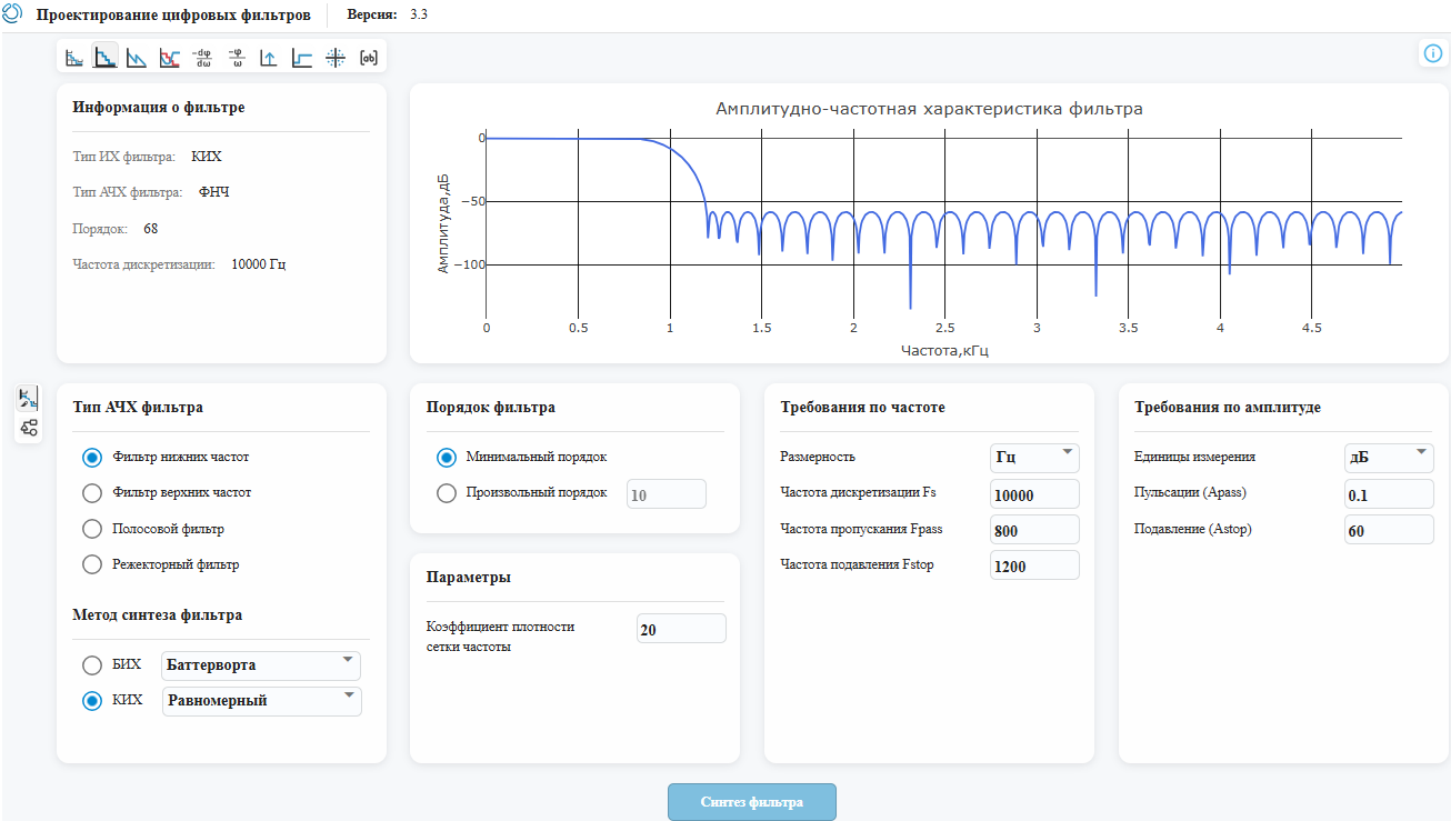
Filter Specification
We know that the spectrum of the original valid signal is limited to 1000 Hz. We also know that the low-pass filter is applied after the operation of adding zeros, which means it operates at an increased sampling rate - in our case, at 10 kHz. It is worth choosing the form of its frequency response so that the bandwidth is approximately limited to 1000 Hz, and at the same time that decent suppression is provided outside the band.
It is also worth considering the filter order. The higher it is, the closer the frequency response shape is to the ideal (rectangular) one, but the large filter order introduces a large delay, and it is also more difficult to implement in hardware. We will establish the following requirements for our low-pass filter:
-
Sampling rate - 10,000 Hz
-
The bandwidth limit is 800 Hz
-
the beginning of the barrier band is 1500 Hz
-
the type of filter is equal-pulsating
-
ripple in the bandwidth - no more than 0.1 dB
-
attenuation in the barrier band - at least 60 dB
-
the filter order is the minimum possible for this specification
The Digital Filter Editor application
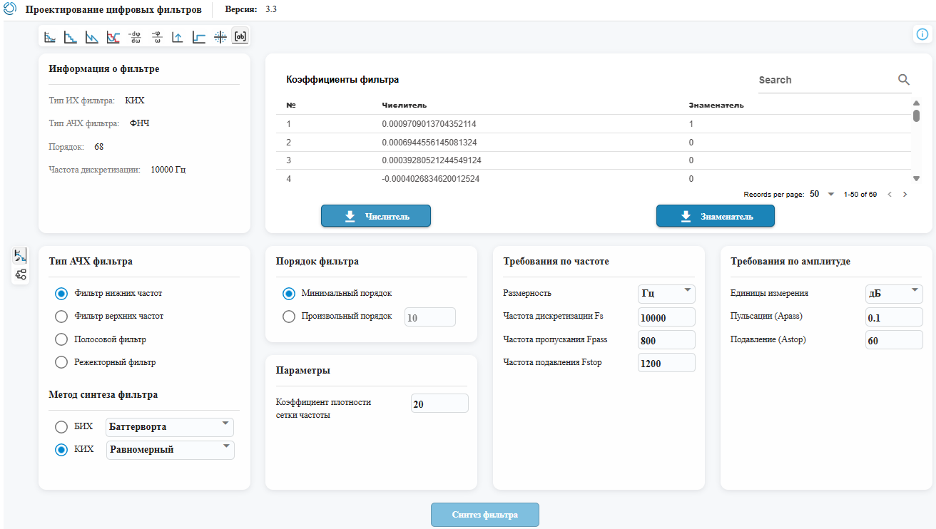
Open the interactive Digital Filter Editor application, set the filter specification, and click the Filter Synthesis button. We observe the shape of the frequency response, as well as the order of synthesized low-frequency - 68:
We can upload the filter coefficients. Since we have synthesized the FIR filter, we are only interested in the coefficients of the numerator of its transfer function. We'll save them to a file. num.txt.
Let's apply a filter to the signal up. To do this, we will transfer the coefficients of the numerator and the signal to the input of the function filter from the EngeeDSP. The result of filtering will be written to a variable up_filtered. Then we will thin this signal with the function downsample, and save the result to a variable decimated.
using DelimitedFiles
b = vec(readdlm("num.txt"));
up_filtered = EngeeDSP.Functions.filter(b,1,up) * L;
decimated = EngeeDSP.Functions.downsample(up_filtered,M);
plot(t, sig, l=:steppost, m=:dot, ms=2, xlim=(0,0.02))
plot!(tM, decimated, l=:steppost, m=:dot, ms=2, legend=false)
We can see that the shape of the sinusoidal signal has been restored. In the time domain, there is a noticeable delay associated with the use of the FIR filter. You can also see that we multiplied the filtering result by the interpolation coefficient. . This was necessary in order not to lose the energy of the signal, which decreased after adding additional zeros.
Let's make sure that the spectral copies in the output signal have been successfully suppressed by the low-pass filter.:
Sdecim, fvec_decim = fftspectrum(decimated, fs*L/M; onesided=true);
plot(fvec_down, Sdown, legend=false)
plot!(fvec_down, Sdecim, lw=3, ylim=(-80,0))
Application of specialized interpolation and decimation functions
The EngeeDSP contains the following functions interp and decimate, which perform operations of increasing and decreasing the sampling frequency along with filtering by automatically synthesized low-pass filter. They do not introduce delays, as they use zero-phase filtering. These functions are useful for analysis and prototyping, but do not reflect the behavior of real sequential DSP systems. However, the coefficients of the synthesized low-pass FIR filter can be extracted from these functions as an additional output argument.
Let's evaluate the result of applying the function interp:
isig, bb = EngeeDSP.Functions.interp(sig,L);
plot(tL, isig, l=:steppost, m=:dot, ms=2, xlim=(0,0.02), legend=false)
dsig = EngeeDSP.Functions.decimate(isig,M);
plot(t, sig, l=:steppost, xlim=(0,0.02), legend=false)
plot!(tM, dsig, l=:steppost, m=:dot, ms=2)
And finally, we will display the impulse response of the automatically calculated low-pass filter.:
plot(bb, l=:stem, m=:c, c=6, mc=14, legend=false, title = "THEIR low-frequency interp functions")
Aliasing effect when the sampling rate is lowered:
In conclusion, we will consider the effect of aliasing, that is, "wrapping" the spectral components of the signal into the first Nyquist zone when the sampling frequency is lowered to such values when the main condition of Kotelnikov's theorem is no longer fulfilled, i.e. when the largest frequency in the signal spectrum goes beyond .
Let's evaluate the effect visually and audibly using the example of a sinusoidal tone with a fundamental frequency of 2.4 kHz. By changing the value of the sampling frequency using a slider, you can observe a change in the fundamental frequency of the tone if the condition of Kotelnikov's theorem is not observed. Starting from the value Hz, the tone will start to decrease:
fs = 6000 # @param {type:"slider",min:3000,max:6000,step:500}
dt = 1/fs;
t = 0:dt:1;
f0 = 2400;
x = sin.(2*pi*f0*t);
S_1, fv_1 = fftspectrum(x, fs; onesided=true);
audioplayer(x,fs)
plot(fv_1, S_1, legend=false, size=(800,200), ylim=(-80,0))
Conclusion
Multi—speed processing is a fundamental tool in DSP that allows you to effectively control the sampling rate of a signal to save computing power, match different digital systems, analyze signals in different frequency bands, and improve conversion quality. Without it, modern communication standards, audio and video codecs would be impossible, and many computing tasks would be unreasonably expensive.
We looked at how to develop prototypes of multi-speed processing systems using functions from the EngeeDSP library.