Kepstra analysis
This example is aimed at comparing the functions of kepstra analysis in Engee and MATLAB. Below are two codes for each of these environments.
In Engee, FFTW packages and standard functions for performing the Fourier transform can be used to perform kepstra analysis.
The following are the functions implemented by us.
using FFTW  # To perform a fast Fourier transform

# Comprehensive capstr
function cceps(x::Vector{Float64})
    X = fft(x,1)                     # The Fourier transform
    p = atan.(imag(X), real(X))
    log_mag = complex.(log.(abs.(X)),p) # Logarithm of the spectrum modulus (adding a small value for stability)
    cepstrum = real(ifft(log_mag,1)) # The inverse Fourier transform
    return cepstrum
end
# Reverse complex kepstr
function icceps(c::Vector{Float64})
    exp_spectrum = exp.(fft(c,1))    # The exponent of the spectrum
    signal = real(ifft(exp_spectrum,1)) # The inverse Fourier transform
    return signal
end
# Valid caption
function rceps(x::Vector{Float64})
    X = fft(x,1)
    log_mag = log.(abs.(X) .+ 1e-10) # The logarithm of the module (with the addition of a stabilizer)
    cepstrum = real(ifft(log_mag))
    return cepstrum
end
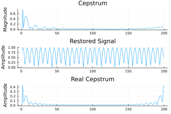
x = sin.(1:0.5:100)  # The input signal

cepstrum = cceps(x)
restored_signal = abs.(icceps(cepstrum))
real_cepstrum = abs.(rceps(x))

# # Visualization
p1 = plot(abs.(cepstrum), title="Cepstrum", ylabel="Magnitude")
p2 = plot(abs.(restored_signal), title="Restored Signal", ylabel="Amplitude")
p3 = plot(abs.(real_cepstrum), title="Real Cepstrum", ylabel="Amplitude")
plot(p1, p2, p3, layout=(3,1), legend=false)
In MATLAB, standard functions can be used to perform kepstra analysis.
- cceps(x) performs a complex cepstr.
- icceps(x) performs an inverse complex cepstr.
- rceps(x) performs a valid cepstr.
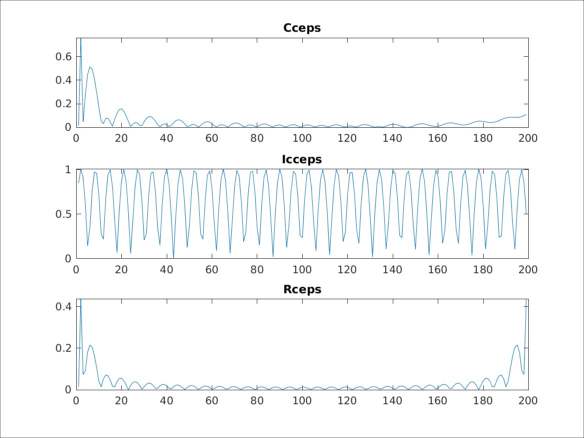
using MATLAB
mat"""
% Complex capstr
ccep = cceps($(x));
% Reverse complex kepstr
iccep = icceps(ccep);
% Valid cap
rcep = rceps($(x));

% Visualization of results
subplot(3,1,1), plot(abs(ccep)), title('Cceps');
subplot(3,1,2), plot(abs(iccep)), title('Icceps');
subplot(3,1,3), plot(abs(rcep)), title('Rceps');
saveas(gcf, 'cep.jpg'); % Сохраняет текущую фигуру как JPG
"""
load("$(@__DIR__)/cep.jpg")
Conclusion
MATLAB has built-in functions for performing these operations. In Engee, you can use third-party libraries for this task, such as DSP or FFTW for more complex signal operations. It is also important to consider that Engee provides more flexibility in how transformations can be implemented. To simplify these operations for your Engee tasks, use the ready-made approaches described in this demo.
Another aspect in comparing the capabilities of the two environments suggests that MATLAB is optimized for working with matrices and signals. However, Engee is generally faster in computing if the code is written taking into account the specifics of this environment, and this gives a significant increase in the speed of execution and testing algorithms in large systems.