Implementation of low- and high-pass filters
This demonstration shows the implementations of two filters defined by the following difference equations:
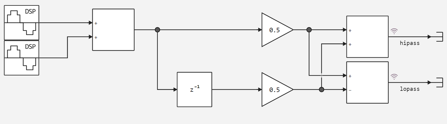
- Low-pass filter: y(n) = 0.5x(n) + 0.5x(n-1) (averaging)
- High-pass filter: y(n) = 0.5x(n) - 0.5x(n-1) (finite difference)
The figure below shows a model from which we can see that common coefficients are given for filters and their main differences are contained in the last adder.
Next, we'll use an auxiliary function to run the model.
function run_model( name_model)

    Path = (@__DIR__) * "/" * name_model * ".engee"

    if name_model in [m.name for m in engee.get_all_models()] # Checking the condition for loading a model into the kernel
        model = engee.open( name_model ) # Open the model
        model_output = engee.run( model, verbose=true ); # Launch the model
    else
        model = engee.load( Path, force=true ) # Upload a model
        model_output = engee.run( model, verbose=true ); # Launch the model
        engee.close( name_model, force=true ); # Close the model
    end
    sleep(5)
    return model_output
end

run_model("hipass_lopass") # Launching the model.
Let's analyze the recorded results by plotting the signals in the time and frequency domains.
hipass = collect(simout["hipass_lopass/hipass"]);
lopass = collect(simout["hipass_lopass/lopass"]);

plot(hipass.time[1:500], [hipass.value[1:500], lopass.value[1:500]],label=["Low-pass filter" "High-pass filter"])
As we can see from the data presented in the time domain, the main differences between the data at the output of the high- and low-pass filters are differences in the amplitude of the signals and the unevenness of the oscillatory pulses, which we observe when using high-pass filters.
using FFTW

Comp_hipass = ComplexF64.(hipass.value);
Comp_lopass = ComplexF64.(lopass.value);

spec_hipass = fftshift(fft(Comp_hipass));
spec_lopass = fftshift(fft(Comp_lopass));

x = [10log10.(abs.((spec_hipass/3e6))),10log10.(abs.((spec_lopass/3e6)))];
plot(x, label =["Low-pass filter" "High-pass filter"])
ylabel!("Power DBW")
xlabel!("Frequency MHz")
Based on the signal spectra, we can see that the filters are working correctly.
Conclusion
In this example, we have analyzed the differences between high-pass filters and low-pass filters using the same coefficients in both cases, thereby showing that there are quite few differences between these filters in terms of implementation.