LFM signal analysis and processing

Introduction

Let's consider a small model containing a block of a linear frequency modulation (LFM) signal generator and a block of a discrete filter with a finite impulse response (FIR filter). In this model, one can visually observe the process of signal transmission, the frequency of which increases linearly during the simulation, through a frequency-selective circuit: a low-pass filter (low-pass filter).

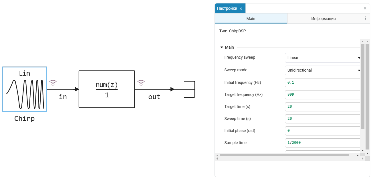
Parameters of the signal source block ChirpDSP The models are shown in the screenshot. We generate a signal whose frequency increases linearly from 0.1 Hz to 999 Hz during 20 seconds of simulation. The signal is discrete, with a sampling frequency of 2 kHz (which allows us to meet the basic condition of Kotelnikov's theorem).

Characteristics of the low-pass filter

Block DiscreteFIRFilter The model stores the coefficients of the numerator of the transfer function of the filter prototype, which we create using functions from the library. DSP.jl. We will specify the 500 Hz filter cutoff frequency, the type of window function for synthesis, and the filter order.:

using DSP;
fs = 2000;
myFIR = digitalfilter(Lowpass(2*500/fs), FIRWindow(hann(32)));

Then we will calculate and display the amplitude-frequency response (frequency response) of the filter to make sure that it is able to transmit only signals with a frequency of no more than 500 Hz.:

myTransferFunction = PolynomialRatio(myFIR,1);
H, w = freqresp(myTransferFunction);
freq_vec = fs*w/(2*pi);
plot(freq_vec, pow2db.(abs.(H))*2, linewidth=3,
     xlabel = "Частота, Гц",
     ylabel = "Амплитуда, дБ",
     title = "АЧХ фильтра нижних частот",
     ylim = (-120, 10))

We use a window filter of the 32nd order, without controlling the sharpness of the transition from the bandwidth to the barrier band. But an attenuation of -6 dB at the 500 Hz limit will suit us. Thus, we have obtained a frequency-selective circuit that allows the low frequencies of our FM signal to pass through.

Simulation of the model

It is worth noting that before launching the model, there is no need to synthesize the low-pass coefficients each time, they are automatically loaded into the discrete filter unit when the model is loaded. And we will observe a visual analysis of the results of LFM signal generation and filtering in the window. Графики interface of the modeling environment.

The main simulation parameters are set so that the calculation and display speed correspond to the "wall clock" - 1 second of simulation is equal to 1 second of elapsed time. And in the graph window, we can observe how, when starting the simulation, the peaks of the spectra of the generated and processed signals move to the right along the frequency axis, while the amplitude of the output signal begins to decrease after passing the 500 Hz mark.

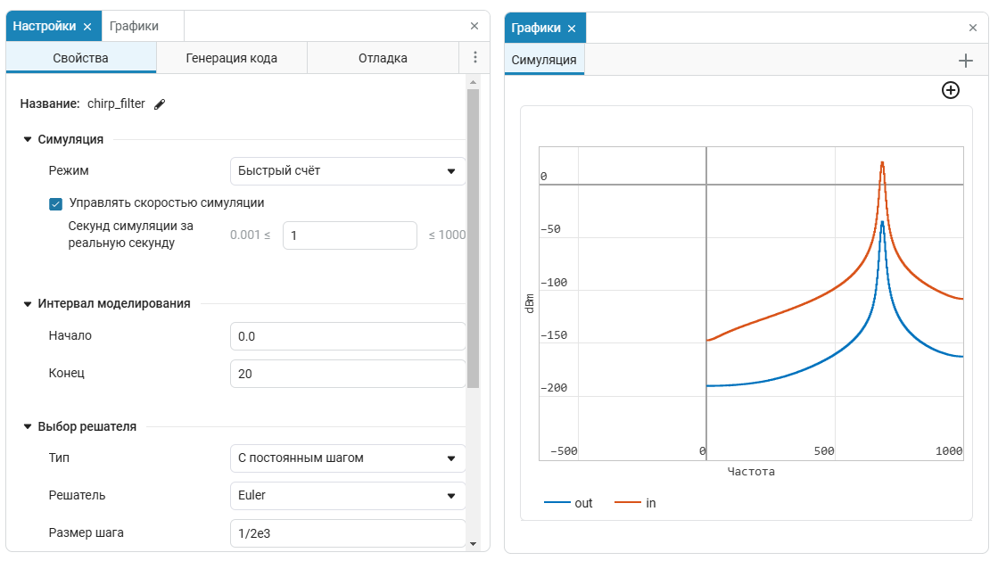
To observe the non-stationary spectrum, we used the built-in signal visualization tool in the frequency domain.

Circuit analysis using an LFM signal

Historically, linearly increasing frequency signals have been used to analyze the frequency response of an unknown circuit. If the amplitude of the FM signal does not change during the observation period, then the shape of the output signal in the time domain reflects the frequency response. Before the development of digital spectral analysis algorithms, such experiments could be carried out using an analog oscilloscope.
In the window Графики let's switch to displaying signals in the time domain. Despite the fact that we are modeling a discrete signal and a digital filter, the principle remains unchanged, and we expect to see a waveform in time reflecting the frequency response of the filter.

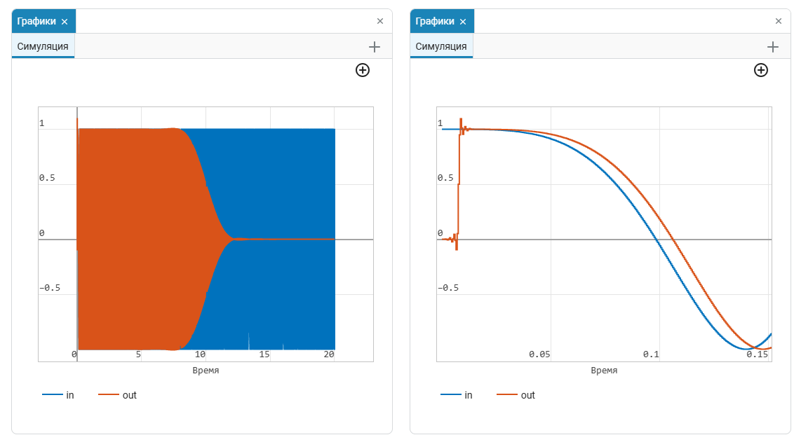
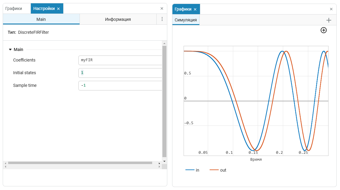
Indeed, after about 10 seconds of simulation, the output signal is suppressed to zero (during which time its frequency reaches 500 Hz). However, if you zoom in on the start time of the simulation, you can observe a delay, a spike, and a beating of the output signal. This is due to the fact that a digital FIR filter will necessarily delay the output signal by its length (filter order, in discrete signal samples), and it also contains certain initial states of its registers. In the default model, the block DiscreteFIRFilter it has zero initial states (parameter Initial states). If we change this value to 1, we will see that now the filter does not need to "catch up" with the sharply changed signal at its input, spikes and beats are not observed.

Conclusion

This model clearly demonstrated the principles of signal generation, the spectrum of which varies over time, visualization of signal spectra using the built-in tools of the modeling environment, and also showed the principle of frequency response analysis of circuits using FM signals.