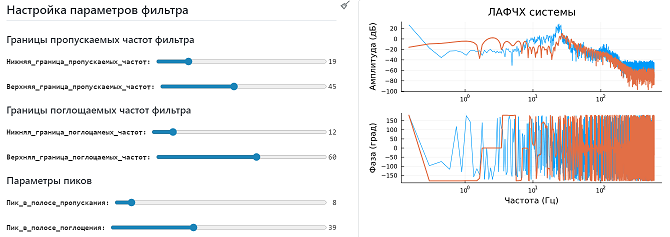
Configuring the filter parameters via a custom form
Let's build a small application (a cell mask) that will help us select filter parameters without leaving the interactive script.
Uploading data
Suppose we have the following signal:
In [ ]:
Pkg.add(["Statistics", "DSP", "CSV"])
In [ ]:
gr()
using CSV, DataFrames
d = CSV.read( "$(@__DIR__)/scope_data.csv", DataFrame );
Let's take the average difference between the time steps as the sampling frequency.
In [ ]:
using Statistics
Fs = 1 / mean(diff(d.Time));    # Sampling rates
Fn = Fs/2;                      # Nyquist Frequency
L = length( d.Time );           # The number of samples in the signal
And let's try to build a filter that meets some technical requirements.
In [ ]:
using FFTW, DSP
Fl = round.(Int, round(L/2)+1)           # The number of points in the discrete Fourier transform
Fv = range(1/Fl, 1, length=Fl) .* Fn;    # Frequency vector (excluding the first point – 0)
Iv = 1:length(Fv);                       # Index vector
In [ ]:
# @markdown ## Configuring filter parameters
# Default values
pT, pB, sT, sB, Rp, Rs = 20, 30, 18, 35, 1, 50;
# @markdown ### The limits of the transmitted filter frequencies
Нижняя_граница_пропускаемых_частот = 19 # @param {type:"slider", min:2, max:100, step:1}
Верхняя_граница_пропускаемых_частот = 45 # @param {type:"slider", min:2, max:100, step:1}
# @markdown ### The limits of the absorbed filter frequencies
Нижняя_граница_поглощамеых_частот = 12 # @param {type:"slider", min:2, max:100, step:1}
Верхняя_граница_поглощаемых_частот = 60 # @param {type:"slider", min:2, max:100, step:1}
# @markdown ### Peak Parameters
Пик_в_полосе_пропускания = 8 # @param {type:"slider", min:2, max:100, step:1}
Пик_в_полосе_поглощения = 39 # @param {type:"slider", min:2, max:100, step:1}
pB, pT = Lower limit of Allowed frequencies, Upper limit of Allowed frequencies
sB, sT = Lower limit of Absorbable frequencies, Upper limit of Absorbable frequencies
Rp = Peak In The Bandwidth
Rs = Peak In The Absorption Band
Wp = (pB, pT) ./ Fn;
Ws = (sB, sT) ./ Fn;
n,Ws = ellipord( Wp, Ws, Rp, Rs); # Let's find the filter order with the desired characteristics
designmethod = Elliptic( n, Rp, Rs ); # Creating an elliptical filter
responsetype = Bandpass( Rp, Rs); # And a bandpass filter
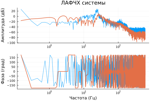
# Smoothed spectrum
TF = fft( d.Measurement ) ./ L
TF1 = filt( digitalfilter(responsetype, designmethod; fs=Fn), TF );
plot(
plot( Fv, 20 .* log10.(abs.([TF[Iv] TF1[Iv]])), xscale=:log10, lw=[1 2] ),
plot( Fv, angle.([TF[Iv] TF1[Iv]]) .* 180/pi, xscale=:log10, lw=[1 2] ),
layout=(2,1)
)
plot!( ylabel=["Amplitude (dB)" "Phase (hail)"], leg=:false )
plot!( title=["LFCH systems" ""], xlabel=["" "Frequency (Hz)"] )
Out[0]:
If you hide code, and set the option "Avtonapovnennya cell, if you change settings" button (the button to the left of the mask cells), it is possible to interactively adjust the filter parameters.
Conclusion
The toolkit of masks for code cells allows you to create your own interface for configuring algorithms. With its help, we can select the filter parameters that will appropriately affect the output signal of a certain link.