Fundamentals of DSP: spectral analysis
In *Digital Signal Processing (DSP) Spectral analysis is a set of methods that make it possible to decompose a signal into frequency components and study its properties in the frequency domain.
The main tasks of spectral analysis in DSP:
-
Determination of the frequency composition of the signal (for example, the allocation of tonal components in the audio signal).
-
Detection of hidden periodicities (for example, vibration analysis in mechanical systems).
-
Filter specification (for subsequent noise removal and useful frequency extraction).
-
Data compression (using frequency representations such as JPEG, MP3).
-
Pattern recognition (for example, speech signal analysis).
The main methods of analysis are:
-
Discrete Fourier transform (DFT) and fast Fourier transform (FFT). Learn more about FFT - in this примере.
-
Periodogram (power spectrum estimation)
-
The Welch method (averaged periodogram)
-
Parametric methods (autoregression, AR)
-
Filter bank
In this example, we will consider the FFT, periodogram, and Welch methods for audio signal analysis.
# This must be done if the necessary libraries are not installed.
# Pkg.add("DSP")
# Pkg.add("WAV")
# Pkg.add("Base64")
# Pkg.add("FFTW")
# Pkg.add("FindPeaks1D")
# Pkg.add("Statistics")
using DSP, WAV, Base64, FFTW, FindPeaks1D, Statistics
The initial signal for analysis
As a test signal, we use an audio recording of a guitar string. Our task is to determine which note is being played by analyzing the spectrum of the signal.
Let's load the numerical samples of the signal with the function wavread, which also allows you to select the sampling frequency of the signal fs.
filename = "$(@__DIR__)/guitar.wav"
audio_data, fs = wavread(filename);
Let's count the number of samples of the signal in the time domain, calculate the time step and form a time vector.:
nsamples = length(audio_data);
dt = 1/fs;
t = 0:dt:((nsamples - 1) .* dt);
sig = vec(audio_data);
We'll use an additional function to listen to audio. audioplayer:
function audioplayer(s, fs);
    buf = IOBuffer();
    wavwrite(s, buf; Fs=fs);
    data = base64encode(unsafe_string(pointer(buf.data), buf.size));
    markup = """<audio controls="controls" {autoplay}>
                <source src="data:audio/wav;base64,$data" type="audio/wav" />
                Your browser does not support the audio element.
                </audio>"""
    display("text/html", markup);
end
Let's listen to the sound of an oscillating string:
audioplayer(sig,fs)
Finally, let's display the signal in the time domain.:
plot(t, sig,
    xguide = "Time, from",
    yguide = "Amlpituda, In",
    title = "Audio signal in time",
    legend = false)
It is possible to find out the fundamental oscillation frequency by the shape of a periodic signal in the time domain, but it is still very difficult.
Estimation of the signal spectrum
Let's consider three methods for constructing a power spectrum or a graph of the spectral power density (SPM) of a test signal. Both metrics are suitable for qualitative analysis of frequency composition.
Let's start by building a power spectrum based on the FFT. Learn more about functions and mathematics - in the previous примере.
A = fft(sig);
B = fftshift(A);
df = fs/nsamples;
freq_vec = -fs/2:df:fs/2-df;
plot(freq_vec, pow2db.(abs.(B.^2)),
    xguide = "Frequency, Hz",
    yguide = "Power, dB",
    title = "Signal power spectrum (based on FFT)",
    xlim = (0,10000),
    legend = false)
A harmonic structure is clearly visible on the spectrum - equally spaced peaks. Harmonics are sinusoidal oscillations whose frequencies are multiples of the fundamental frequency. .
- the lowest frequency in the signal (the first harmonic), and the higher harmonics are frequencies of the form , where (second, third, etc.).
Periodogram
Periodogram is a method for estimating spectral power density (SPM) a signal based on its discrete Fourier transform (DFT). In practice, it is calculated using FFT.
Algorithm:
-
A segment of the signal is taken (for example, 1024 samples).
-
The FFT of this segment is calculated.
-
The amplitude spectrum is squared and normalized by the sample length.
-
A frequency power graph is obtained.
p1 = DSP.periodogram(sig, onesided=true, fs=fs);
plot(freq(p1), pow2db.(power(p1)),
    xguide = "Frequency, Hz",
    yguide = "Power/frequency, dB/Hz",
    title = "Spectral power density of the signal (periodogram)",
    xlim = (0,10000),
    legend = false)
However, this method has a number of disadvantages.:
-
High variance – the estimate jumps with small data changes.
-
Leakage of the spectrum (leakage) – due to the finite length of the signal, false frequencies occur (solved by window functions, for example, Hanna or Hamming).
-
Low frequency resolution – if the signal is short, the nearby frequencies merge.
The Welch method
The Welch method is a modification of the periodogram in which:
-
The signal is split into overlapping segments.
-
A window function is applied to each segment (for example, Hanna, Hamming) - this reduces the effect of spectrum leakage.
-
A periodogram is calculated for each segment.
-
The results are averaged → the variance is reduced.
p2 = DSP.welch_pgram(sig, onesided=true, fs=fs);
plot(freq(p2), pow2db.(power(p2)),
    xguide = "Frequency, Hz",
    yguide = "Power/frequency, dB/Hz",
    title = "Spectral density of signal power (Welch method)",
    xlim = (0,10000),
    legend = false)
Determining the fundamental frequency of the signal
Let's focus on the evaluation of the SPM using the Welch method and analyze the low frequency range (from 0 to 1500 Hz). We will find the ** peaks** in the spectrum - they correspond to the harmonics of the signal. The function will help us with this. findpeaks1d from the corresponding package. Let's select the first six harmonics and display them on the graph.:
spectrum = pow2db.(power(p2));
fvec = freq(p2);
pkindices, properties = findpeaks1d(spectrum;
                                    height = -65,
                                    prominence = 20);
plot(fvec, spectrum,
    linewidth = 3,
    xguide = "Frequency, Hz",
    yguide = "Power/frequency, dB/Hz",
    title = "Peaks of the signal spectrum (Welch method)",
    xlim = (0,1500),
    label = "spectrum")
scatter!(fvec[pkindices], spectrum[pkindices]; color="red", markersize=5, label="peaks")
The very first peak is at 219 Hz. But we can also programmatically determine the frequencies of the first six harmonics and find the average distance between them in Hz. It is this estimate that we will take as the fundamental frequency.:
harmonics = fvec[pkindices[1:6]]
base_freq = mean(diff(harmonics))
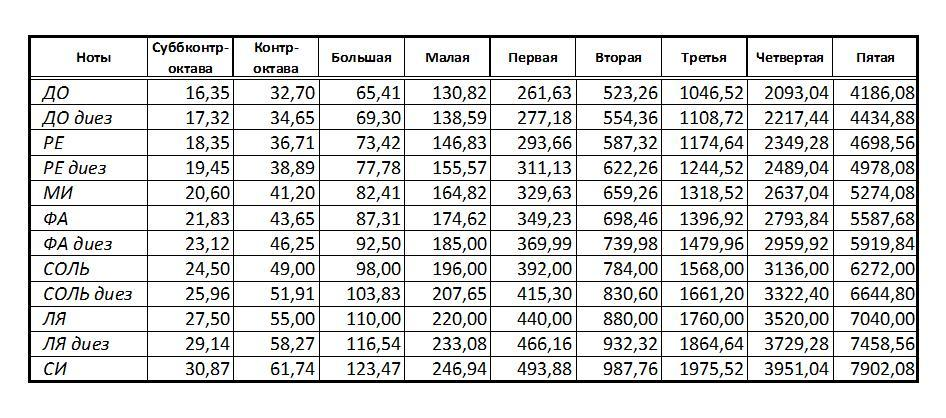
According to the table, the note played is A minor octave La.
Selecting the first harmonic
We synthesize a simple elliptical low-pass filter (low-pass filter) that suppresses frequencies above 300 Hz. This will allow us to cut off the higher harmonics. Let's filter out the original signal and listen to the result.:
myfilt = digitalfilter(Lowpass(2*300/fs), Elliptic(10, 0.1, 80));
clean220 = filt(myfilt, sig);
audioplayer(clean220 * 2, fs)
We hear a more "pure" tone, devoid of color. It is not immediately possible to recognize the guitar in it, since it is the higher harmonics that give the timbre to the instrument.
Conclusion
We examined three standard methods for estimating the signal spectrum - the FFT, the periodogram, and the Welch method using the example of analyzing the frequency composition of an audio signal from an oscillating guitar string - and also determined the fundamental frequency of the oscillation.