Fractional delay with Farrow filter

The Farrow filter is a digital interpolation filter that can be used to oversample (change the sampling rate) signals with a non—integer coefficient. It was proposed by Chris Farrow in 1988.

How does the Farrow filter work?

The input signal is divided into segments (usually 4 samples for cubic interpolation).
For each new value, a polynomial approximation is calculated between samples.
The position of the new reference is determined by a fractional delay (for example, between x[n] and x[n+1]).
The output is a signal with a new sampling frequency.

In this example, we will consider the use of the Farrow filter to implement fractional delay of signals, which is especially useful in digital signal processing (DSP), telecommunications, radar and audio systems.

Fractional delay is the shift of a signal by a fractional number of samples (for example, by 0.5, 0.73 or 1.25 from the sampling period).

The whole delay (1, 2, 3…) is easily implemented by a FIFO buffer.
Fractional delay requires interpolation between samples, and the Farrow filter helps here.

The example describes two implementations of block models of the Farrow filter - the first and the third order. In general, the structure is based on FIR filters and an interpolation polynomial scheme.:

Implementation of Farrow filters in the model

Model fractional_delay.engee It contains two subsystems of Farrow filters. Subsystem Первый_порядок implements a simple linear interpolation scheme:

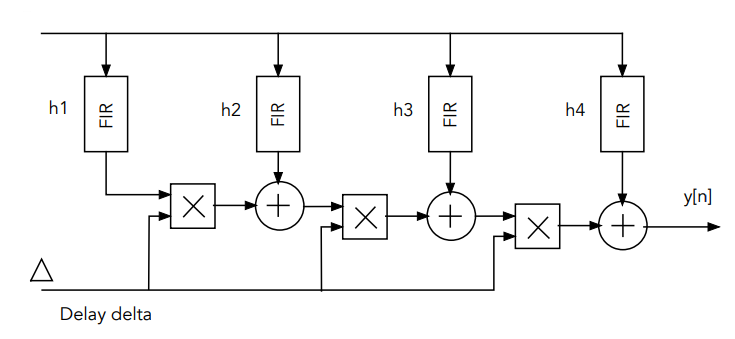
While the subsystem Третий_порядокIt is more similar to the general structure of Farrow, and contains three FIR filters.:

Moreover, the second and third FIR filters are implemented in the form of blocks. Дискретный КИХ-фильтр signal processing libraries, and the first one is in the form of a subsystem, where the direct structure of an inversely symmetric FIR filter is assembled from primitive arithmetic elements.:

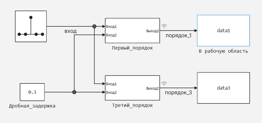
The general model considers the passage of a 50 Hz sinusoidal signal through two subsystems at a sampling frequency of 1000 Hz with a fractional delay factor of 0.3 periods:

On the time domain graphs, you can see that the linear filter (1st order) successfully introduces a fractional delay of 0.3 periods. This is clearly visible in the area of the passage of sinusoids through zero. The 3rd-order filter has a more complex structure and introduces an additional group delay of 1 period - the resulting delay is 1.3 periods.:

Analysis of the frequency response of Farrow filters

If both filters can handle the task of introducing fractional delay, then what is affected by the complexity of the filter structure and order?

To do this, we need to analyze their frequency characteristics. One of the methods of analysis is to supply a single pulse to the input of a linear stationary system (filter). In this case, the output of the filter will reflect its impulse response, from which it is easy to switch to the amplitude-frequency response (frequency response). Auxiliary model fractional_delay_impulse.engeeIt has a discrete pulse source block as a signal source, and also contains two blocks В рабочую область to automate filter analysis with library functions DSP.jl:

Let's use the automatic model launch function.:

function start_model_engee()
    try
        engee.close("fractional_delay_impulse", force=true) # закрытие модели 
        catch err # в случае, если нет модели, которую нужно закрыть и engee.close() не выполняется, то будет выполнена её загрузка после catch
            m = engee.load("$(@__DIR__)/fractional_delay_impulse.engee") # загрузка модели
        end;

    try
        engee.run(m, verbose=true) # запуск модели
        catch err # в случае, если модель не загружена и engee.run() не выполняется, то будут выполнены две нижние строки после catch
            m = engee.load("$(@__DIR__)/fractional_delay_impulse.engee") # загрузка модели
            engee.run(m, verbose=true) # запуск модели
        end
end

start_model_engee (generic function with 1 method)

start_model_engee();

Building...
Progress 0%
Progress 100%
Progress 100%

Let's collect the output data (pulse characteristics of the filters) and plot their frequency response:

using DSP
fs = 1000;
dataframe1 = collect(data1);
dataframe3 = collect(data3);
b1 = dataframe1.value;
b3 = dataframe3.value;
farrow_1 = PolynomialRatio(b1, 1);
farrow_3 = PolynomialRatio(b3, 1);
H1, w1 = freqresp(farrow_1);
H3, w3 = freqresp(farrow_3);
freq_vec = fs*w1/(2*pi);
plot(freq_vec, pow2db.(abs.(H1))*2, 
                    linewidth=3, 
                    title = "АЧХ фильтров Фарроу", 
                    xguide = "Частота, Гц",
                    label = "Линейный фильтр")
plot!(freq_vec, pow2db.(abs.(H3))*2, 
                    linewidth=3, 
                    yguide = "Амплитуда, дБ",
                    label = "3-й порядок")

As you can see, as the filter order increases, its linearity increases and the bandwidth expands. Small-order filters can only successfully handle low-frequency signals, while higher-order filters can operate over a wide frequency range of incoming signals.

Conclusion

Advantages of the Farrow filter for fractional delay:

Flexibility — any fractional delay can be set (0.1*, 0.75 and so on).
\ , Moderate computational complexity — requires fewer resources than SINC interpolation.
*Good quality - Cubic interpolation provides better accuracy than linear interpolation.

Applying fractional delay:

Synchronization in digital communication (clock signal tuning).
Audio Effects (smooth pitch-shifting, phase correctors).
Radar and sonar systems (precise time alignment of signals).
Adaptive filters (delay adjustment in noise cancellation systems).

The Farrow filter is an efficient way to implement fractional delay with a balance between accuracy and computational cost. It is especially useful in tasks where smooth delay change is required without loss of signal quality.