Phase-locked frequency when receiving an FM signal
In this example, we will assemble an FM signal receiver based on phase-locked frequency (PLL). We investigate the capture of a noisy signal, the restoration of modulation and ripple at the output. The model consists of Engee base blocks, so all internal loop signals are available.
The FM signal is given by the expression
The carrier has a frequency of 10 Hz, and the modulating signal — glad/s. The modulation index .
The phase detector multiplies the input signal and the oscillator signal:
The filter suppresses the component of the doubled carrier. With a small phase difference, the detector coefficient . The loop uses two low-pass and a PI controller.:
where with, , .
The linearized loop model has transfer functions
At the modulation frequency determines the gain and phase shift of the reconstructed signal.
Calculation of loop characteristics
Calculate the modulation index, the suppression of the doubled carrier, and the loop response at 0.5 Hz.
using Main: engee, plot, plot!, histogram, hline!, savefig, Animation, frame, gif
Kd = 0.5                 # phase detector coefficient, 1/rad
τ = 0.02                 # the time constant of each low-pass filter, with
Kp, Ki = 15.0, 100.0     # PI controller coefficients
ω0 = 62.8319             # carrier frequency, rad/s
Am, Ω = 1.5, π           # frequency deviation amplitude and modulation frequency, rad/s

pll_F(s) = 1 / (τ * s + 1)^2         # two consecutive low-pass
pll_C(s) = Kp + Ki / s               # The PI controller
pll_L(s) = Kd * pll_F(s) * pll_C(s) / s      # open loop: GONG integrates frequency into phase
pll_H(s) = pll_L(s) / (1 + pll_L(s))         # from the deviation of the input frequency to the control signal

β = Am / Ω
ripple = Kp * Kd * abs(pll_F(2im * ω0))   # the amplitude of the component is 2ω0 after filters and Kp
Hm = pll_H(im * Ω)

println("The modulation index β = ", round(β, digits = 3))
println("Attenuation of the 2ω0 component by two low-pass: ", round(abs(pll_F(2im * ω0)), digits = 3))
println("Estimation of 2ω0 ripples in the control signal: ", round(ripple, digits = 2), " рад/с")
println("|H| at the modulation frequency: ", round(abs(Hm), digits = 3),
        ", фаза ", round(rad2deg(angle(Hm)), digits = 1), "°")
At the modulation frequency, the calculation gives a gain of about 1.2 and a phase shift of about -4°. At the frequency of the double carrier, 20 Hz, the filters pass about 14% of the amplitude. Therefore, noticeable ripples are expected at the output.
Description of the model
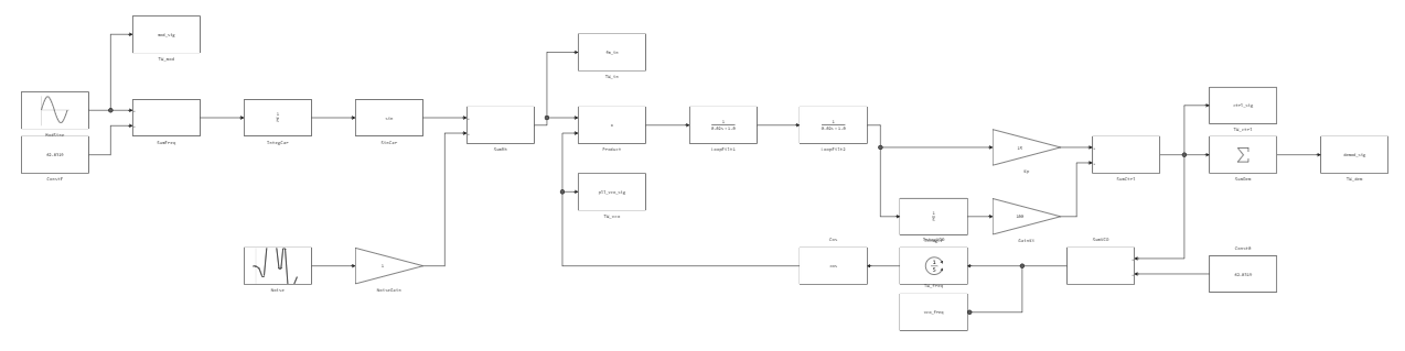
The model contains the following parts:
[PIPE] Part of the loop [PIPE] Engee Blocks [PIPE]
[PIPE]---[PIPE]---[PIPE]
[PIPE] FM source and noise [PIPE] Sine Wave, Integrator, Random Number [PIPE]
[PIPE] Phase detector [PIPE] Product [PIPE]
[PIPE] Filters and a PI controller [PIPE] Transfer Fcn, Gain, Integrator [PIPE]
[PIPE] Controlled generator [PIPE] Integrator, Trigonometric Function [PIPE]
[PIPE] Recording of signals [PIPE] To Workspace [PIPE]
The calculation step is 0.5 ms, the simulation time is 6 s. We analyze the modulation, the output of the demodulator, the input of the receiver, the signal of the generator and its frequency control.
Download the model from the example folder and run the calculation.
using Statistics

model_name = "PLL_FM"
model_file = joinpath(@__DIR__, "PLL_FM.engee")

model = engee.load(model_file; force=true)

# Running the simulation; the To Workspace signals will appear in the workspace
engee.run(model)
We will receive signals from the To Workspace blocks.
# To Workspace stores the signal as a table: time, value.
function signal_data(signal)
    table = collect(signal)
    return table[!, 1], table[!, 2]
end

t_mod,  x_mod  = signal_data(Core.eval(Main, :(mod_sig)))
t_fm,   x_fm   = signal_data(Core.eval(Main, :(fm_in)))
t_vco,  x_vco  = signal_data(Core.eval(Main, :(pll_vco_sig)))
t_dem,  x_dem  = signal_data(Core.eval(Main, :(demod_sig)))
t_ctrl, x_ctrl = signal_data(Core.eval(Main, :(ctrl_sig)))
t_freq, x_freq = signal_data(Core.eval(Main, :(vco_freq)))

omega0 = 62.8319
freq_deviation = x_freq .- omega0

println("Number of counts: ", length(t_mod))
println("Duration: ", last(t_mod), " with")
println("RMS mod_sig: ", round(sqrt(mean(x_mod .^ 2)), digits=4))
println("RMS demod_sig: ", round(sqrt(mean(x_dem .^ 2)), digits=4))
12001 counts are recorded. The RMS value of the modulation is close to 1.06 rad/s; the output of the demodulator also contains loop ripples.
After receiving the data, we will close the model.
engee.close(model_name; force = true)
Let's compare the modulation and output of the demodulator, the input signal and the oscillator, as well as the frequency control and deviation.
# 1. Modulating and demodulated signals.
p1 = plot(
    t_mod, x_mod;
    label="Modulation",
    linewidth=2,
    ylabel="The amplitude",
    title="Modulating and demodulated signals",
    legend=:topright, legendfontsize=8, xlabel="Time, from",
    grid=true
)
plot!(
    p1, t_dem, x_dem;
    label="Demodulator output",
    linewidth=1.5,
    linestyle=:dash
)

# 2. FM signal and short-range VCO signal.
p2 = plot(
    t_fm, x_fm;
    label="FM input signal",
    linewidth=1.2,
    xlims=(2.0, 2.4),
    ylabel="The amplitude",
    title="FM signal and VCO",
    legend=:topright, legendfontsize=8, xlabel="Time, from",
    grid=true
)
plot!(
    p2, t_vco, x_vco;
    label="GOON",
    linewidth=1.2,
    linestyle=:dash
)

# 3. Control signal and VCO frequency deviation.
p3 = plot(
    t_ctrl, x_ctrl;
    label="Control signal",
    linewidth=2,
    ylabel="рад/с",
    title="VCO Management",
    legend=:topright, legendfontsize=8, xlabel="Time, from",
    grid=true
)
plot!(
    p3, t_freq, freq_deviation;
    label="Frequency deviation",
    linewidth=1.2,
    linestyle=:dash
)

# 4. Enlarged fragment of the PLL reaction.
p4 = plot(
    t_mod, x_mod;
    label="Modulation",
    linewidth=2,
    xlims=(2.0, 4.0),
    ylabel="The amplitude",
    title="The PLL reaction",
    legend=:topright, legendfontsize=8, xlabel="Time, from",
    grid=true
)
plot!(
    p4, t_dem, x_dem;
    label="Demodulator output",
    linewidth=1.5,
    linestyle=:dash
)

plot(
    p1, p2, p3, p4;
    layout=(2, 2),
    size=(1400, 1050)
)
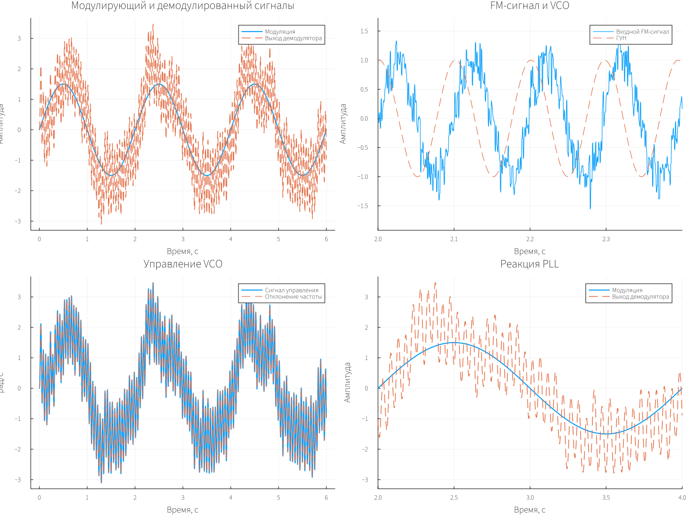
The output repeats the modulation with a frequency of 0.5 Hz. Pulsations of about 20 Hz are visible on top of it — the component of the doubled carrier. The signal of the generator is in quadrature with the input, and the control corresponds to the deviation of its frequency.
Let's estimate the amplitudes after the end of the transition process, starting from 2 s.
# The amplitude of the harmonic frequency f (Hz) in the signal x(t) in the section t ≥ t_start
function harmonic_amplitude(t, x, f; t_start = 2.0)
    mask = t .>= t_start
    tt, xx = t[mask], x[mask]
    c = sum(xx .* cos.(2π * f .* tt))
    s = sum(xx .* sin.(2π * f .* tt))
    return 2 * hypot(c, s) / length(tt)
end

a_mod = harmonic_amplitude(t_mod, x_mod, 0.5)
a_dem = harmonic_amplitude(t_dem, x_dem, 0.5)
a_2f0 = harmonic_amplitude(t_dem, x_dem, 20.0)

println("mod_sig, 0.5 Hz:   ", round(a_mod, digits = 3), " рад/с")
println("demod_sig, 0.5 Hz: ", round(a_dem, digits = 3), " рад/с; отношение ", round(a_dem / a_mod, digits = 3),
        " (теория |H| = ", round(abs(Hm), digits = 3), ")")
println("demod_sig, 20 Hz:  ", round(a_2f0, digits = 3), " рад/с")
@assert length(t_mod) > 100 && all(isfinite, x_dem)
string("PLL FM passed; samples=", length(t_mod), "; modulation gain=", round(a_dem/a_mod; digits=3))
The measured gain at the modulation frequency is about 1.17, which is close to the calculation. The remaining 20 Hz component is associated with limited filter suppression. By changing their parameters and the coefficients of the PI controller, it is possible to study the effect of the loop band on demodulation.
Conclusion
The PLL monitors the FM signal and restores the modulation with a gain of about 1.17, close to the calculated one. The residual pulsations of the doubled carrier show the effect of the loop filters on the quality of demodulation.